Supervised Learning - Prediction Week 3 Challenge
1A-
Gradient descent is an optimization technique that can find the minimum of an objective function. It is a greedy technique that finds the optimal solution by taking a step in the direction of the maximum rate of decrease of the function.
By contrast, Gradient Ascent is a close counterpart that finds the maximum of a function by following the direction of the maximum rate of increase of the function.
To understand how gradient descent works, consider a multi-variable function f(w)f(w), where w=[w1,w2,…,wn]Tw=[w1,w2,…,wn]T. To find the ww at which this function attains a minimum, gradient descent uses the following steps:
-
Choose an initial random value of ww
-
Choose the number of maximum iterations
T -
Choose a value for the learning rate η∈[a,b]η∈[a,b]
-
Repeat following two steps until ff does not change or iterations exceed T
a.Compute: Δw=−η∇wf(w)Δw=−η∇wf(w)
b. update ww as: w←w+Δww←w+Δw
The left arrow symbol being a mathematically correct way to write an assignment statement.
Here ∇wf∇wf denotes the gradient of ff as given by:
∇wf(w)=[∂f(w)∂w1 ∂f(w)∂w2 ⋮ ∂f(w)∂wn]
2A-
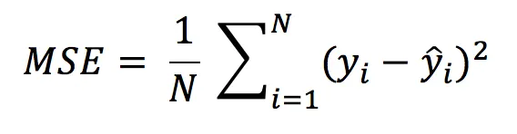
Mean Square Error(MSE)
MSE is calculated by the sum of square of prediction error which is real output minus predicted output and then divide by the number of data points. It gives you an absolute number on how much your predicted results deviate from the actual number. You cannot interpret many insights from one single result but it gives you a real number to compare against other model results and help you select the best regression model.
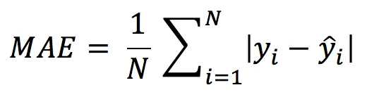
Mean Absolute Error(MAE) is similar to Mean Square Error(MSE). However, instead of the sum of square of error in MSE, MAE is taking the sum of the absolute value of error.
3A- the different loss functions for regression are listed given below:
Root mean square error, mean squared error,mean absolute error.
4A-The learning rate controls how quickly the model is adapted to the problem. Smaller learning rates require more training epochs given the smaller changes made to the weights each update, whereas larger learning rates result in rapid changes and require fewer training epochs.
we deals with 2 parameters:
- Machine learnable parameters – The parameters that the algorithms learn/estimate on their own during training for a particular dataset
- Hyper-parameters are variables that machine learning engineers or data scientists provide precise values to regulate how algorithms learn and modify the model’s performance
5A-Model evaluation is very important in data science. It helps you to understand the performance of your model and makes it easy to present your model to other people. There are many different evaluation metrics out there but only some of them are suitable to be used for regression. This article will cover the different metrics for the regression model and the difference between them. Hopefully, after you read this post, you are clear on which metrics to apply to your future regression model.R Square/Adjusted R Square is better used to explain the model to other people because you can explain the number as a percentage of the output variability. MSE, RMSE, or MAE are better be used to compare performance between different regression models.
A positive coefficient indicates that as the value of the independent variable increases, the mean of the dependent variable also tends to increase. A negative coefficient suggests that as the independent variable increases, the dependent variable tends to decrease.
6A-The fundamental point is that when you add predictors to your model, the multiple Rsquared will always increase, as a predictor will always explain some portion of the variance. Adjusted Rsquared controls against this increase, and adds penalties for the number of predictors in the model
R-squared and adjusted R-squared enable investors to measure the performance of a mutual fund against that of a benchmark. Investors may also use them to calculate the performance of their portfolio against a given benchmark.