Supervised Learning - Prediction Week 3 Challenge

Q1.

Gradient descent is an iterative optimization algorithm used to minimize a function. In machine learning, it is typically used to minimize the loss function (which measures the error between predictions and actual values).

Let us define the y_predicted as:

y_predicted = mx + b

where m, b are constants.

The MSE is defined as M

$$MSE=\frac{1}{n}\sum _{i=1}^n{(y_a-(mx+b))}^2$$

To find the local minima, the gradient of MAE wrt to b and m is calculated:

Gradient with respect to b:

$$\frac{\mathrm{\partial }MSE}{\mathrm{\partial }b}=\frac{2}{n}\sum _{i=1}^n(-1)(y_a-(mx+b))$$

Gradient with respect to m:

$$\frac{\mathrm{\partial }MSE}{\mathrm{\partial }m}=\frac{2}{n}\sum _{i=1}^n(-x)(y_a-(mx+b))$$

Update rule for b:

$$b = b - \text{learning\_rate} \cdot \frac{\partial MSE}{\partial b}$$

Update rule for m:

$$m=m-\text{learning\_rate}\cdot \frac{\mathrm{\partial }MSE}{\mathrm{\partial }m}$$

Let us consider the below dataset for performing gradient descent:

x = [1,2,3,4,5]

y = [2,4,6,8,10]

The loss function to be used is the mean square error which is defined as:

MSE=n∑i=1(ya−yp)2n${\displaystyle MSE=\sum _{i=1}^n\frac{{(y_a-y_p)}^2}{n}}$yp

n = total number of data points

y_p =predicted outcome

${\displaystyle {\mathrm{==y}}_p}$ y_a= actual outcome

After 15,944 iterations, the values of b and m are found to be 0.00234 and 1.99935 respectively. Hence, the predicted values are determined using equation:

y_predicted=1.99935x+0.00234

(code is in ipynb file attached)

---

---

Q2.

The two major loss functions are:

Mean Absolute Error

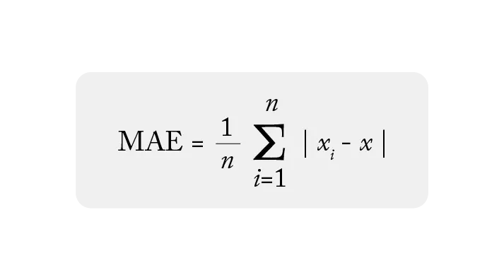
n=total number of data points

x_i= predicted outcome

x= actual outcome

Mean Square Error

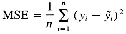
n=total number of data points

y_i= predicted outcome

y'_i= actual outcome

The gradient descent performed using MAE is known as L1 norm whereas the gradient descent using MSE is known as L2 norm.

L1 vs L2 differences

• As L1 involves absolute error, the error obtained for outlier data points is smaller as compared to the mean square error. As the aim of the gradient descent method is to reduce error/loss function, MAE or L1 norm is preferred for data set with outliers
• The loss function when calculated using L2 or MSE is convex function and this ensures global minima is determined for most cases. On the other hand, using L1 norms, the model may converge at local minima thus resulting in poor prediction of outputs

---

---

Q3.

The different loss functions are:

• Mean Absolute Error

MAE=∑ni=1|yp−ya|n${\displaystyle MAE=\frac{\sum _{i=1}^n|y_p-y_a|}{n}}$

• Mean Square Error

MSE=∑ni=1(yp−ya)2n${\displaystyle MSE=\frac{\sum _{i=1}^n{(y_p-y_a)}^2}{n}}$

• Root mean square error

RMS=√∑ni=1(yp−ya)2n

---

---

Q4.

In gradient descent method, the error function is minimized by calculating the tangent at the weights and moving along the convex function in incremental steps. The size of these steps is determined by the learning rate.

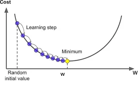
A larger value of learning rate could results in overshooting of the weights and could result in inaccurate value of minima. On the other hand, a smaller value of learning rate improves the accuracy of the algorithm but results in increased computational expenditure.

---

---

Q5.

Evaluation of linear regression helps you to understand the performance of your model. There are three major metrics used to evaluate regression model
R² and adjusted R²

MSE , RMSE and MAE

`R² and adjusted R² are better used to explain the model to other people because you can explain the number as a percentage of the output variability. On the other hand, the other two metrics are used to choose the best amongst the various regression models.

MSE gives a larger error value and may be difficult for comparison of different algorithms. In such cases, it is beneficial to opt for RMSE as the error values are smaller and the dimensionality of the predicted value is same as the actual values.

Furthermore, MSE penalizes significantly the outlier data points as compared to MAE. Hence, based on the scenario where outliers points need not be penalized significantly, we choose MAE over MSE.

---

---

Q6.

When the linear regression involves one dependent variable and one independent variable, the regression model is evaluated by
${\displaystyle R^2}$R²or coefficient of determination. In case of a data set with one dependent variable and several independent variable, the model is evaluated using multiple coefficient of determination.

When the regression model is not influenced by some of the independent variables, we opt for adjusted coefficient of determination. Any addition of data point where the independent variable can be ignored does not affect the value of R².

R2adjusted=1−(1−R2)(n−1)n−k−1${\displaystyle R_{adjusted}^2=1-\frac{(1-R^2)(n-1)}{n-k-1}}$MSE=1nn∑i=1(ya−(mx+b))2

n= number of data points

k= number of independent variables