Supervised Learning - Prediction Week 3 Challenge

2)Difference between L1 & L2 Gradient descent method

Ans2)

Mean Absolute Error, L1-(MAE) is another loss function used for regression models. MAE is the sum of absolute differences between our target and predicted variables. So it measures the average magnitude of errors in a set of predictions, without considering their directions. The range is also 0 to ∞.

MAE=(1n)n∑i=1∣∣yi−ypi∣∣MAE=(1n)∑i=1n|yi-yip|

Mean Squared Error, L2-(MSE) is the most commonly used regression loss function. MSE is the sum of squared distances between our target variable and predicted values.

MSE=(1n)n∑i=1(yi−ypi)2MSE=(1n)∑i=1n(yi-yip)2

Since MSE squares the error (y — y_predicted = e), the value of error (e) increases a lot if e > 1. If we have an outlier in our data, the value of e will be high and e² will be >> |e|. This will make the model with MSE loss give more weight to outliers than a model with MAE loss.

3)What are the different loss functions for regression

1. Mean Square Error, Quadratic loss, L2 Loss

Mean Squared Error (MSE) is the most commonly used regression loss function. MSE is the sum of squared distances between our target variable and predicted values.

Below is a plot of an MSE function where the true target value is 100, and the predicted values range between -10,000 to 10,000. The MSE loss (Y-axis) reaches its minimum value at prediction (X-axis) = 100. The range is 0 to ∞.

2. Mean Absolute Error, L1 Loss

Mean Absolute Error (MAE) is another loss function used for regression models. MAE is the sum of absolute differences between our target and predicted variables. So, it measures the average magnitude of errors in a set of predictions, without considering their directions. The range is also 0 to ∞.

3. Huber Loss, Smooth Mean Absolute Error

Huber Loss is less sensitive to outliers in data than the squared error loss. It’s also differentiable at 0. It’s basically an absolute error, which becomes quadratic when the error is small. How small that error has to be to make it quadratic depends on a hyperparameter, 𝛿 (delta), which can be tuned. Huber loss approaches MAE when 𝛿 ~ 0 and MSE when 𝛿 ~ ∞ (large numbers.).

The choice of the delta is critical because it determines what you’re willing to consider as an outlier. Residuals larger than delta are minimized with L1 (which is less sensitive to large outliers), while residuals smaller than delta are minimized “appropriately” with L2.

One big problem with using MAE for the training of neural nets is its constantly large gradient, which can lead to missing minima at the end of training using gradient descent. For MSE, the gradient decreases as the loss gets close to its minima, making it more precise.

Huber loss can be really helpful in such cases, as it curves around the minima which decreases the gradient. And it’s more robust to outliers than MSE. Therefore, it combines good properties from both MSE and MAE. However, the problem with Huber loss is that we might need to train the hyperparameter delta which is an iterative process.

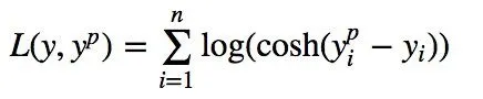
4. Log-Cosh Loss

Log-cosh is another function used in regression tasks that’s smoother than L2. Log-cosh is the logarithm of the hyperbolic cosine of the prediction error.

5. Quantile Loss

In most real-world prediction problems, we are often interested to know about the uncertainty in our predictions. Knowing about the range of predictions as opposed to only point estimates can significantly improve decision-making processes for many business problems.

Quantile loss functions turn out to be useful when we are interested in predicting an interval instead of only point predictions. Prediction interval from least square regression is based on an assumption that residuals have constant variance across values of independent variables. We cannot trust linear regression models which violate this assumption. We cannot also just throw away the idea of fitting the linear regression model as a baseline by saying that such situations would always be better modelled using non-linear functions or tree-based models. This is where quantile loss and quantile regression come to the rescue as regression-based on quantile loss provides sensible prediction intervals even for residuals with non-constant variance or non-normal distribution.

4. What is the importance of the learning rate?

Learning rate (λ) is one such hyper-parameter that defines the adjustment in the weights of our network with respect to the loss gradient descent. It determines how fast or slow we will move towards the optimal weights.

The Gradient Descent Algorithm estimates the weights of the model in many iterations by minimizing a cost function at every step.

Learning rate is a scalar, a value that tells the machine how fast or how slow to arrive at some conclusion. The speed at which a model learns is important and it varies with different applications. A super-fast learning algorithm can miss a few data points or correlations which can give better insights into the data. Missing this will eventually lead to wrong classifications.

And, to find the next step or the adjacent data point, the gradient descent algorithms multiply the gradient by learning rate (also called step size).

For example, if the gradient magnitude is 1.5 and the learning rate is 0.01, then the gradient descent algorithm will pick the next point 0.015 away from the previous point.

If a learning rate is too small, learning will take too long.

And if a learning rate is too large, the next point will perpetually bounce haphazardly across the bottom of the valley.

How to evaluate linear regression

There are three main errors (metrics) used to evaluate models, mean absolute error, Mean Squared error and R2 score.

1. MAE

MAE is the sum of absolute differences between our target and predicted variables. So, it measures the average magnitude of errors in a set of predictions, without considering their directions. (If we consider directions also, that would be called Mean Bias Error (MBE), which is a sum of residuals/errors). The range is also 0 to ∞. The lesser the MAE better the line fits all the data points.

2. MSE

Mean Squared Error(MSE) is the sum of squared distances between our target variable and predicted values. MAE is similar to MAE but the errors are squared.

3. R- Squared

R-Squared is the ratio of Sum of Squares Regression (SSR) and Sum of Squares Total (SST). Sum of Squares Regression is the amount of variance explained by the regression line. R-squared value is used to measure the goodness of fit. The greater the value of R-Squared, the better is the regression model.

R-Squared is also termed as the coefficient of determination. For the training dataset, the R2R2 bounded between 0 and 1, but it can become negative for the test dataset if the SSE is greater than SST. If the value of R-Squared is 1, the model fits the data perfectly with a corresponding MSE = 0.

Here is a visual representation to understand the concepts of R-Squared in a better manner.

Note that the greater the value of SSR, the more is the variance covered by the regression / best fit line out of total variance (SST). R-Squared can also be represented using the following formula:

R-Squared = 1 – (SSE/SST)

6. What is the difference between multiple and adjusted coefficients of determination

R² measures the proportion of the total variation in Y explained by the regression model.

Here are some key points about R²:

• It is a non-negative quantity with a range 0 ≤ R² ≤ 1
• R² = 0 implies that the regression line does not fit the data at all.
• R² = 1 implies that the regression line is a perfect fit.

Adjusted R² is a modified version of R² adjusted with the number of predictors. It penalizes for adding unnecessary features and allows a comparison of regression models with a different number of predictors. The adjusted R-squared increases only if the new term improves the model more than would be expected by chance. It decreases when a predictor improves the model by less than expected by chance.

Obtaining a negative value for Adjusted R² can indicate few or all of the following:

• The linear model is a poor fit for the data
• The number of predictors is large
• The number of samples is small