Supervised Learning - Prediction Week 3 Challenge

Q.1 Linear regression-Perform Gradient Descent in Python with any loss function

• Let y= mx+b is an eqaution of line,here x= dependent variable,x=independent variable,m= slope and b= intercept.
• we are going to use this eqaution to train our model and with given dataset and predict the value of x for any value of x.
• our Aim is to find the values of m,b such that line corresponding to those values is the best fiting line or gives minimum error.
• As we discussed in above,to calculate m&c at minimum error, we are are calculating error by using mean sqaured error function
• `mse = (1/n)sum_(i=1)^n(Y_a-Y_p)^2`,where `Y_a`= Actaul value ,`Y_p`= predicted value,n= number of data points.
• Putting, predicted value=Y_p`= (mx_i+b)
• `mse = (1/n)sum_(i=1)^n(Y_a-(mx_i+b))^2`
• In above we have defined the mean sqaured error function or we can called it Cost function.now lets get into next main part to minimizing the error and finding m&b.
• The Gradient descent Algorithm
• Let us use Gradient descent method to minimize the loss function,It optimization algorithm.it's based on convex function and tweaks its parameters iteratively to minimize the loss function to its local minimum.
• Steps to apply gradient descent -

1.Initially let m=0,b=0 and L= 0.001 , here L= learning rate.This controls the how much value of m changes

with each step.

2.To find the local minima ,let us Calculate the partial derivative of the loss function with respect to m,

and plug in the current values of x, y, m and c in it to obtain the derivative value `D_m`.

• `D_m = (1/n)sum_(i=1)^n(2(y_a-(mx_i +b))(-x)`
• `D_m = (-2/n)sum_(i=1)^n(x)(y_a-y_p)`
• Similarly lets find the partial derivative with respect to b, Db :
• `D_c= (-2/n)sum_(i=1)^n(y_a-y_p)`

3. Now we update the current value of m and c using the following equation:

• `m= m- L times D_m`
• `c=c-L timesD_c`
• We repeat this process until our loss function is a very small value or ideally 0 (which means 0 error or 100% accuracy). The value of m and c that we are left with now will be the optimum values.

Let us implement Gradient descent in python .

import numpy as np
import matplotlib as pyplot as plt

np.random.seed(0)
x=np.random.rand(100,1)
y=2+3*x+np.random.rand(100,1)

#scatter plot 
plt.scatter(x,y,s=20)
plt.xlabel('x')
plt.ylabel('y')
plt.show()

slope=0
intercept=0
learning_rate = 0.01
n=len(y)
mse_L =[]
iteration_L=[]
for j in range(0,100):
    for i in range(0,n):
        y_p = slope*x+intercept
        mse=(1/n)*(sum([val**2 for val in (y-y_p)]))
        d1=-2/n*sum(x*(y-y_p))
        d2=-2/n*sum(y-y_p)
        slope=slope-learning_rate*d1
        intercept=intercept-learning_rate*d2
        mse_L.append(mse)
        iteration_L.append(j)
print("slopes="+str(slope))
print("intercept="+str(intercept))
print("iteration="+str(j))
print("mse="+str(mse))

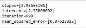
• Results: slope,intercept & error

• Result visualization

plt.plot(iteration_L,mse_L)
plt.xlabel('no_of_iteration')
plt.ylabel('Cost_function')
plt.show()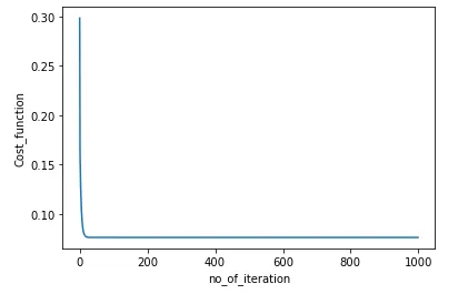

• Scatter plot

plt.scatter(x,y,s=20)
plt.xlabel('x')
plt.ylabel('y')
plt.show()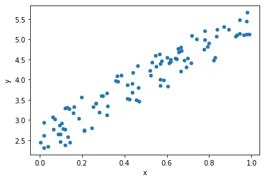

• Best fit line

plt.scatter(x,y,s=20)
plt.plot([min(x),max(x)],[min(y_p),max(y_p)],color='r')
plt.show()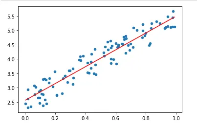

• In this way,after iteration=999, we minimized error upto [0.07623325] and we have obtained values of slope=[2.93655106] & intercept=[2.55808002] and line corresponding to these values is the best fit line.
• Note : Above coding file in ipynb format is submitted

Q.2 Difference between L1 & L2 Gradient descent method

L1 = Mean Absolute Error

L2 = Mean Squared error

Mean Absolute Error(MAE):

• Mean absolute error,also known as L1 loss.
• It is calculated by taking the absolute difference between the predicted values and the actual values and averageing it across the dataset.
• MAE measures only the magnitude and doesn't concern itself with their diection.
• The lower the MAE, higher the accuracy of model.
• `MAE = (1/n)sum_(i=1)^n abs(Y_a-Y_p)`,where Y_a= Actaul value ,Y_p = predicted value, n = sample size`

Pros:

• It is easy to calculate evaluation metric.
• All the errors are weighted on the same scale since absolute values are taken.
• It is useful if the training data has outliers as MAE does not penalize high errors caused by outliers.

Cons:

• Sometimes the large errors coming from the outliers end up being treated as the same as low error.
• It can be challenging to compute gradient in MAE.

Mean Squared Error(MSE):

• MSE is one of the most common regression loss functions.In mean sqaured error also known as L2 loss.
• It can calculated by sqauring the difference between the predicted value and averaging it across the dataset.
• MSE is also known as Quadratic loss as the penalty is not proporational to the error but to the sqaure of error.
• sqauring the error gives higher weight to the outliers,which results in a smooth gradient for small error.
• MSE will never be negative since the errors are sqaured.The value of the error ranges from zero to infinity.
• A good model will have an MSE value closer to zero.
• `MSE = (1/n)sum_(i=1)^2(Y_a-Y_p)^2`

Pros:

• MSE values are expressed in quadratic eqautions.Hence when we plot it,we get gradient descent with only one global minima.
• For small errors,it converges to the minima efficiently.there are no local minima.
• MSE penalize the model for having huge errors by sqauring them.
• It is particularly helful in weeding out outliers with large errors from the model by putting more weight on them.

Cons:

• One of the main advantages of MSE becomes a disadvantages when there is bad prediction.the sensitivity to outliers magnifies the high errors by sqauring them.
• When a new outlier is introduced into the data,the model will try to take in the outlier.By doing so it will produce a different line of best fit which may cause the final result to skewed.

Q.3 What are the different loss functions for regression

• Loss functions for regression

1.Mean Absolute error(MAE)

• Mean absolute error,also known as L1 loss.
• It is one of the most simple yet robust loss functions used for regression models.
• It is calculated by taking the absolute difference between the predicted values and the actual values and averageing it across the dataset.
• MAE measures only the magnitude and doesn't concern itself with their direction.
• The lower the MAE, higher the accuracy of model.
• `MAE = (1/n)sum_(i=1)^n abs(Y_a-Y_p)`,where Y_a= Actaul value ,Y_p = predicted value, n = sample size`
• Regression problems may have variables that are not strictly Gaussian in nature due to the presence of outliers (values that are very different from the rest of the data). MAE would be the ideal option in such case,because It does not take into account the direction of outliers.

2.Mean sqaured error(MSE)

• MSE is one of the most common regression loss functions.mean sqaured error also known as L2 loss.
• It almost Every data scientist’s preference when it comes to loss functions for regression.This is because most variables can be modeled into a Gaussian distribution.
• It can calculated by sqauring the difference between the predicted value and averaging it across the dataset.
• MSE is also known as Quadratic loss as the penalty is not proporational to the error but to the sqaure of error.
• sqauring the error gives higher weight to the outliers,which results in a smooth gradient for small error.
• MSE will never be negative since the errors are sqaured.The value of the error ranges from zero to infinity.
• A good model will have an MSE value closer to zero.
• `MSE = (1/n)sum_(i=1)^2(Y_a-Y_p)^2`

3.Huber Loss

• Now we know that the MSE(L2 Loss) is great for learning outliers while the MAE(L1 Loss) is great for ignoring them. But what about something in the middle?
• L1 loss is more robust than its counterpart.
• L1 loss is less stable than L2 loss.
• Huber Loss combines the robustness of L1 with the stability of L2, essentially the best of L1 and L2 losses. For huge errors, it is linear and for small errors, it is quadratic in nature.
• Huber Loss is characterized by the parameter delta (𝛿). For a prediction f(x) of the data point y, with the characterizing parameter 𝛿, Huber Loss is formulated as:
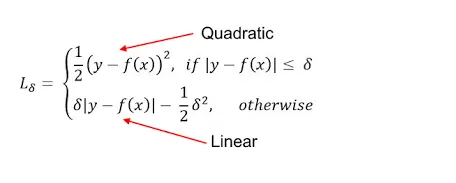
• What is the equation says is : For Loss values less than delta,use the MSE;For Loss values greater than delta,use the MAE.This effectively combines the best of worlds from two loss functions.

Q.4 What is the importance of learning rate

• Solutions for most machine learning problems are achieved by gradient descent algorithm.
• Gradient descent algorithm involves reducing the cost function. The cost function can be anything like cross entropy, mean square error.
• Cost function is relation between the predicted output and actual output. We have to minimize the cost function because we want the difference of them to be minimal.
• In Gradient descent method,The Cost function is minimized by calculating tangent at the weights and moving along convex function in increamental steps.The size of steps is determined by the Learning rate.

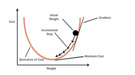
• It is denoted by L or `alpha`

Effect of different Values for learning rate

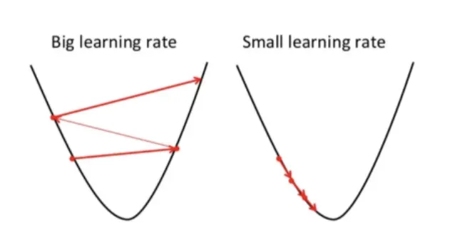
• Learning rate represents the size of the steps our optimization algorithm takes to reach the global minima. To ensure that the gradient descent algorithm reaches the local minimum we must set the learning rate to an appropriate value, which is neither too low nor too high.
• The learning rate should be an optimum value. If the learning rate will be high, the steps taken will be large and we can miss the minima. As a result, the model will never reach the optimal value for the cost function.
• On the other hand, if the learning rate will be too small, The model will take too much time to reach the minimum cost.

Q.5 How to evaluate linear regression

• Evaluation of linear regression help us to understand performance of models.and for that Evaluation metrices are used.
• Evaluation metrics are a measure of how good a model performs and how well it approximates the relationship.
• Let us look at some Evaluation metrices :-MAE, MSE, RMSE,R-squared and Adjusted R-squared.
• we are going to use scikit learn to evaluate the linear regression .

Importing neccessary libraries

import numpy as np
import matplotlib.pyplot as plt
import pandas as pd

Reading & Understanding data

marketing = pd.read_csv('tvmarketing.csv') #reading csv file

#disaplying first 5 rows
marketing.head()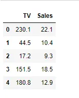 

#displaying last 5 rows
marketing.tail()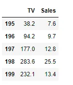

#checking column
marketing.info()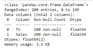

#getting some statstical insights from dataframe
marketing.describe()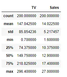

Visvulization of data

#Scatterplot
marketing.plot(x='TV',y='Sales',kind='scatter')

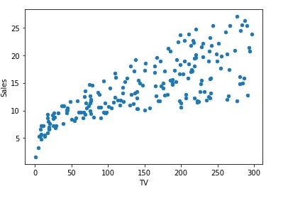
Seperating independent and dependent variables

x = marketing['TV']
x.head()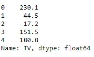

y = marketing['Sales']
y.head()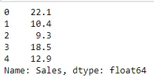

Splitting data into training and test set

from sklearn.model_selection import train_test_split
x_train,x_test,y_train,y_test = train_test_split(x,y,train_size =0.7,random_state= 0)

x_train.shape ,x_test.shape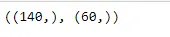

#reshaping

x_train = x_train.values.reshape(-1,1) 

x_test = x_test.values.reshape(-1,1)

#Checking shape after reshaping
x_train.shape ,x_test.shape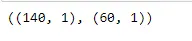

Performing linear regression

#import linear regression from sklearn

from sklearn.linear_model import LinearRegression

lr = LinearRegression()       # model initialization

lr.fit(x_train,y_train)       # Fit the data to train

• Coefficients Calculation

#Print the intercept and coefficients
print('slope=',lr.coef_)
print('intercept=',lr.intercept_)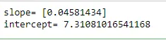

• Predictions

y_pred = lr.predict(x_test) 

Linear Regression Model Evaluation

1.Mean Absolute error(MAE)

• `MAE = (1/n)sum_(i=1)^n abs(Y_a-Y_p)`,where `Y_a`= Actaul value ,`Y_p`= predicted value,n= number of data points.

from sklearn.metrics import mean_absolute_error
print("MAE:",mean_absolute_error(y_test,y_pred))

2.Mean sqaured error(MSE)

• `mse = (1/n)sum_(i=1)^n(Y_a-Y_p)^2`,where `Y_a`= Actaul value ,`Y_p`= predicted value,n= number of data points.

from sklearn.metrics import mean_squared_error
print("MSE:",mean_squared_error(y_test,y_pred))

3.Root Mean sqaured error(RMSE)

• `rmse = sqrt((1/n)sum_(i=1)^n(Y_a-Y_p)^2)`,where `Y_a`= Actaul value ,`Y_p`= predicted value,n= number of data points.

print("RMSE:",np.sqrt(mean_squared_error(y_test,y_pred)))

4. R squared(R2)

• `SS_(RES)`=Sum sqaured regression error ,`SS_(TOT)`=Sum sqaured total error

from sklearn.metrics import r2_score
r2 = r2_score(y_test,y_pred)
print('R2_score:',r2)

5. Adjusted R Squared

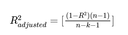
• In the equation above, n is the number of data points ,k is the number of indepenent variables in model

n=200
k=1
adj_r2_score = 1 - ((1-r2)*(n-1)/(n-k-1))
print('Adj_R2_score:',adj_r2_score)

• Note : Above coding file in ipynb format is submitted

Q.6 What is the difference between multiple and adjusted coefficient of determination

1. R squared(R2):-

• It measures the proportion of the variation in your dependent variable explained by all of your independent variables in the model
• It assumes that every independent variable in the model helps to explain variation in the dependent variable.
• In reality, some independent variables (predictors) don't help to explain dependent (target) variable. In other words, some variables do not contribute in predicting target variable.
• Mathematically, R-squared is calculated by
• 
• `SS_(RES)`=Sum sqaured regression error ,`SS_(TOT)`=Sum sqaured total error
• R-Squared is also called coefficient of determination.
• Its values between 0% and 100%. A R-squared value of 100% means the model explains all the variation of the target variable.And a value of 0% measures zero predictive power of the model.
• For example:When R-sqaured value is 0.9 means our model is capable to exaplain 90 % of variance of data.

2. Adjusted R-Squared:-

• It measures the proportion of variation explained by only those independent variables that really help in explaining the dependent variable. It penalizes you for adding new feature(independent variable) that do not help in predicting the dependent variable.
• Adjusted R-squared value can be calculated based on value of r-squared, number of independent variables (predictors), total sample size.

• In the equation above, n is the number of data points ,k is the number of indepenent variables in model

Difference between R-square and Adjusted R-square:-

1. When we add a independent variable to a model, the R-squared increases, even if the independent variable is insignificant. It never declines. Whereas Adjusted R-squared increases only when independent variable is significant and affects dependent variable.

• For Example:

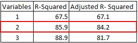
• In above table, adjusted R- square is maximum when we included two variables. It declines when third variable is added. Whereas R - Squared increases when we added third variable. It means third variable is insignificant to the model

2. Adjusted R-squared can be negative when R-squared is close to zero.

3. Adjusted R-squared value always be less than or equal to R-squared value.