Supervised Learning - Prediction Week 3 Challenge

Que. 1 Perform Gradient Descent in Python with any loss function

Ans. Gradient descent is an optimization algorithm used to minimize a loss function in the context of machine learning. A simple example of gradient descent in Python using a quadratic loss function is given; In this example, I defined a simple quadratic loss function (loss_function) and its derivative (gradient). The gradient_descent function performs the gradient descent optimization, and visualize the convergence by plotting the parameter values (x_values) against the corresponding loss values (losses).

Que.2 Difference between L1 & L2 Gradient descent method

Ans. L1 and L2 regularization are two different methods used in the context of gradient descent to prevent overfitting by adding a regularization term to the loss function. Here are the main differences between L1 and L2 regularization:

a) Regularization Term:

L1 Regularization (Lasso): Adds the absolute values of the coefficients as a penalty term to the loss function.

L2 Regularization (Ridge): Adds the squared values of the coefficients as a penalty term to the loss function.

b) Effect on Model Parameters:

L1 Regularization: Tends to produce sparse weight vectors, i.e., it encourages some of the weights to be exactly zero. This can be useful for feature selection as it effectively ignores less important features.

L2 Regularization: Tends to shrink the weights towards zero, but rarely results in exactly zero weights. It often leads to a more evenly distributed set of weights.

c) Geometric Interpretation:

L1 Regularization: The regularization term has the shape of a diamond (L1 norm), which intersects the contour lines of the loss function at the coordinate axes. The solution is likely to be on one of the axes.

L2 Regularization: The regularization term has the shape of a circle (L2 norm), and the solution tends to be towards the center of the circle.

d) Robustness to Outliers:

L1 Regularization: Generally more robust to outliers because it can ignore less important features by setting their weights to zero.

L2 Regularization: Can be sensitive to outliers since it considers the square of the weights, which amplifies the effect of large weights.

e) Computational Complexity:

L1 Regularization: Often leads to solutions with some weights being exactly zero, which can simplify the model and reduce the number of features considered.

L2 Regularization: Generally results in smaller weights but rarely exactly zero, which might involve all the features in the final model.

Que.3 What are the different loss functions for regression?

Ans. Here are some widely used regression loss functions:

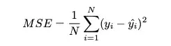
Mean Squared Error (MSE):

The most common loss function for regression.

It penalizes large errors more than small ones.

Formula:

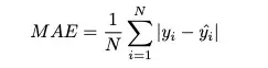
Mean Absolute Error (MAE):

Measures the average absolute difference between the true and predicted values.

Less sensitive to outliers compared to MSE.

Formula:

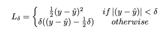
Huber Loss:

A combination of MSE for small errors and MAE for large errors.

It is less sensitive to outliers than MSE.

It has a tunable parameter δ that determines the threshold for switching between MSE and MAE.

Formula:

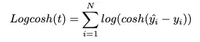
Log-Cosh Loss:

A smooth approximation of Huber loss.

It is differentiable and provides a compromise between MSE and MAE.

Formula:

Quantile Loss (Pinball Loss):

Used for quantile regression, which is useful when you want to predict different quantiles of the target distribution.

The loss is asymmetric and encourages the model to focus on a specific quantile.

Formula:

Que.4 What is the importance of learning rate?

Ans. The learning rate plays a crucial role in the training process of machine learning models. It requires careful consideration and tuning to strike the right balance between convergence speed, accuracy, and stability. Experimenting with different learning rates and monitoring the training process is often necessary to find an optimal value for a given task.

Here are some key points regarding the importance of the learning rate:

Convergence: A learning rate that is too small may cause the optimization process to converge very slowly. The model takes small steps toward the optimal solution at each iteration, and it may require a large number of iterations to reach convergence.

On the other hand, a learning rate that is too large can cause the optimization process to oscillate or diverge.

Speed of Convergence:

The learning rate directly affects how quickly the model converges to the optimal solution.

Accuracy and Generalization:

The learning rate can impact the accuracy of the model and its ability to generalize to new, unseen data.

Stability and Robustness:

A well-tuned learning rate contributes to the stability and robustness of the training process.

Hyperparameter Tuning:

The learning rate is a hyperparameter that needs to be tuned along with other hyperparameters to achieve optimal model performance.

Adaptive Learning Rates:

In some optimization algorithms, adaptive learning rates are used to automatically adjust the learning rate during training based on the observed behavior of the optimization process.

Que.5 How to evaluate linear regression.

Ans. Evaluating the performance of a linear regression model involves assessing how well the model fits the data and makes predictions.

Here are common methods for evaluating linear regression models:

Coefficient of Determination (R-squared): R-squared measures the proportion of the variance in the dependent variable that is predictable from the independent variables.

The value of R-squared ranges from 0 to 1, with higher values indicating better model fit.

However, R-squared does not necessarily indicate the model's predictive accuracy.

Mean Squared Error (MSE) or Root Mean Squared Error (RMSE):

• MSE measures the average squared difference between the predicted and actual values.
• RMSE is the square root of MSE and is in the same units as the dependent variable.
• Lower values of MSE or RMSE indicate better predictive performance.

Mean Absolute Error (MAE):

• MAE measures the average absolute difference between the predicted and actual values.
• Like RMSE, lower values of MAE indicate better predictive performance.
  

Residual Analysis:

• Examine the residuals (the differences between predicted and actual values).
• Plot residuals against predicted values to check for patterns or heteroscedasticity.
• A scatter plot of residuals should ideally show no discernible pattern.

Distribution of Residuals:

Check if the residuals are normally distributed. A histogram or Q-Q plot can help assess this.

Cross-Validation:

Use cross-validation to assess how well the model generalizes to new data.

Split the dataset into training and testing sets, fit the model on the training set, and evaluate on the testing set.

These methods provide different perspectives on the performance of the linear regression model. It's advisable to use a combination of these metrics and visualizations to thoroughly evaluate the model's strengths and weaknesses.

Que.6 What is the difference between multiple and adjusted coefficient of determination

Ans.

1. Multiple Coefficient of Determination ( 2R2):

Purpose: Measures the proportion of the variance in the dependent variable that is explained by the independent variables in the model.

Calculation: 2=1−SSRSSTR 2=1− SSTSR

where SSR is the sum of squared residuals (the differences between observed and predicted values) and SST is the total sum of squares (a measure of the total variance in the dependent variable).

Interpretation: 2R2

ranges from 0 to 1, where 0 indicates that the model explains none of the variance, and 1 indicates perfect explanation of the variance.

2. Adjusted Coefficient of Determination ( adj2R adj2):

Purpose: Similar to 2R2, but it penalizes the use of additional independent variables that do not significantly contribute to the model.

Calculation: adj2=1−(1− 2)⋅( −1) − −1R adj2=1− n−k−1(1−R 2)⋅(n−1)

​where n is the number of observations and k is the number of independent variables.

Interpretation: Like 2R2, adj2R adj2

​ranges from 0 to 1. Higher values indicate a better fit, but adj2R adj2

​tends to be lower than 2R2

if unnecessary variables are included in the model.