Supervised Learning - Prediction Week 3 Challenge

1.Perform Gradient Desecent in Python with any loss function.

Gradient Descent : It is an iterative optimization algorithm to find the minimum of a function, the function is our loss function, it work on the linear regression approach as we all know the basic linear equation of line is Y=mx+c using this equation and iterate our model to find the best fit line and evaluate the Y value by identifying the best value of m and c where m is the slope and c is the y intercept.

Mean Squared Error Function : To evaluate the m and c values the Mean Squared Error Function(MSE) is taken the steps as follows;

1. Difference between Y(actual) and Y(predicted) = Y-Yp

2. Square the differences = (Y-Yp)^2

3. find the mean of the squares = 1/n Σ(Y-Yp)^2

E=1/nΣ(Y-(mx+c))^2

Define m= 0 and c=0 as initial conditions

take learning rate as 0.0001

Then calculate the partial derivative of the above error w.r.t m and c

md = 1/nΣ2(Y-(mx+c)) * (x)

md = -2/nΣ x *(Y-Yp)

cd = -2/nΣ(Y-Yp)

4. Then update the current value of m & c using the equations

m= m-L*md

c= c-L*cd

a loop is created till the loss function is minimum

import numpy as np
import matplotlib.pyplot as plt

x = np.array([2, 3, 4, 5, 6])   # defining x array
y = np.array([10, 20, 30, 40, 50])    # defining y array
m = 0   # initial conditions
c = 0   # initial conditions
iteration = 1000
n = len(x)
learning_rate = 0.0001

for i in range (iteration):
    y_pred = m * x + c
    md = -2/n * sum(x*(y-y_pred))  # Partial derivative of y_pred w.r.t m
    cd = -2/n * sum(y-y_pred)      # Partial derivative of y_pred w.r.t c
    m = m - learning_rate * md     # evaluating m
    c = c - learning_rate * cd     # evaluating c
    print("m{}, c{}, iteration{}".format(m,c,i))

# plotting the results
plt.rcParams['figure.figsize'] = (12.0,9.0)
y_pred = m*x + c
plt.scatter(x, y)
plt.plot([min(x), max(x)], [min(y_pred), max(y_pred)], color = 'red')
plt.show()

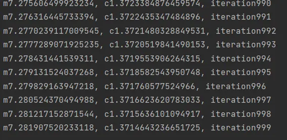
The optimized value of m and c for the above program is shown for 1000 iterations

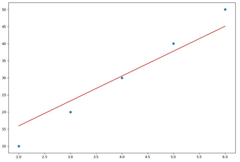
The results are plotted as shown above for best fit

From the above gradient descent algorithm the value of m=7.281 and c=1.3714

2. Difference between L1 & L2 gradient descent method.

The regression losses of gradient descent method L1 & L2 represents the Mean Absolute Error(MAE) & Mean Square Error (MSE)

Mean Absolute Error (MAE)/L1 loss:

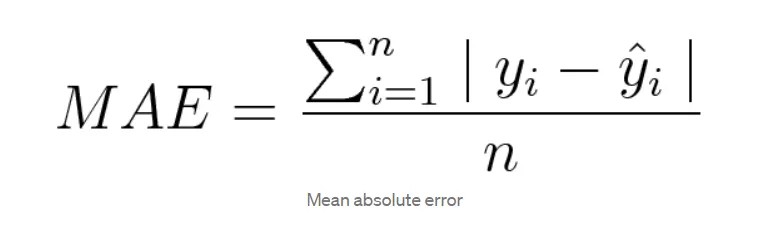
y(i) - actual value
y_cap(i) - Predicted value

mean absolute error is measured as the mean of sum of difference between actual value and predicted value, it measures the magnitude of error but not their direction like MSE,but unlike MSE, MAE is complicated and more robust to outliers since it does not use the squaring

Mean Square Error/L2 loss:

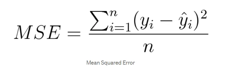
y(i) - actual value
y_cap(i) - Predicted value

Mean Square Error is measured as the average of squared difference between actual and prediction, it is concerned with the average magnitude then their direction and due to squaring, predictions which are far away from actual values are deviated heavily in comparison to less deviated predictions, it is easier to calculate the gradients.

3. what are the different loss functions for regressions?

• Mean Sqaure Error(MSE)

y(i) - actual value
y_cap(i) - Predicted value

n - number of observations

• Mean Absolute Error (MAE)

y(i) - actual value
y_cap(i) - Predicted value

n - number of observations

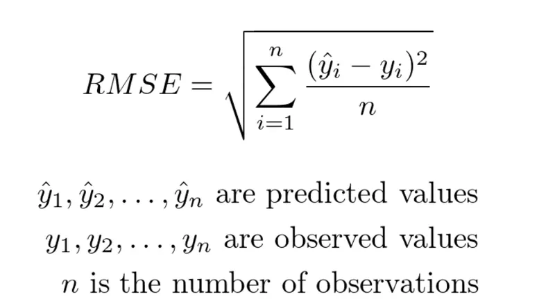
• Root Mean Square Error(RMSE)

• Mean Bias Error

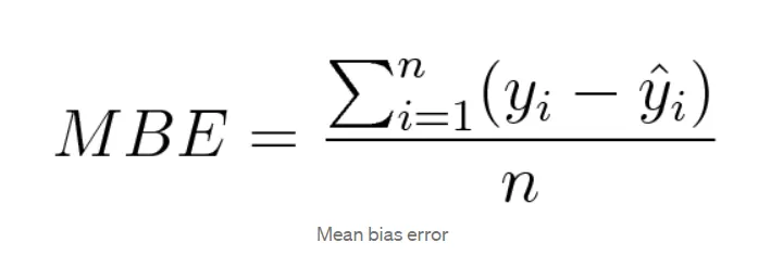
y(i) - actual value
y_cap(i) - Predicted value

n - number of observations

4. What is the importance of learning rate?

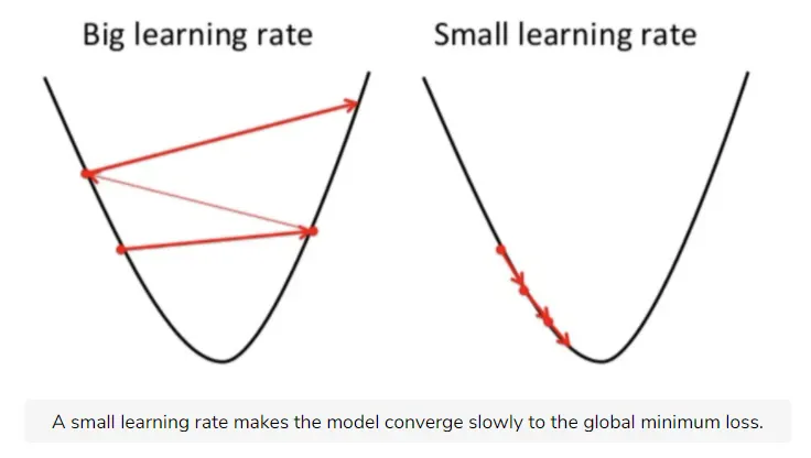
The learning rate in the descent algorithm is used as a tuning parameter to optimize the algorithm, that determines the step size of each iteration, too high learning rate results in difficulty in convergence and may show divergent behaviour in calculating loss functions and too low learning rate progresses slowly and makes small updates in the algorithm,and takes lot of time to converge

5. How to evaluate linear regression?

Linear regression can be evaluted by following metrices

• R^2 and adjusted R^2

R^2 measures how much variations in the dependent variable of model is explained, it is the square of correlation coefficient R.

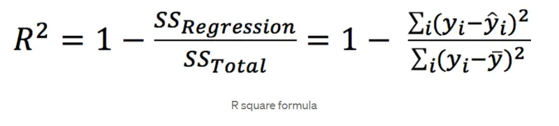
R Square is calculated by the sum of squared of prediction error divided by the total sum of the square which replaces the calculated prediction with mean. R Square value is between 0 to 1 and a bigger value indicates a better fit between prediction and actual value.R Square is a good measure to determine how well the model fits the dependent variables.If the model has many independent variable there will be a problem of overfitting to reduce the overfiting problem adjusted R^2 is introduced.

Mean Square Error(MSE) It gives you an absolute number on how much your predicted results deviate from the actual number,Root Mean Square Error (RMSE) is the sqaure root of the MSE, RMSE used widely since MSE calculated by squaring of errors and RMSE calculated by rooting of the squared error brings it back to the same level of prediction error,which makes it easier for interpretation.Mean absolute error (MAE) measures the error based on their weights but not on their direction.

6. What is the difference between multiple and adjusted coefficient of determination?

If the regression model involves single dependent variable and single independent variable, the model is evaluated using R^2 regression, if it has single dependent varaible and multiple independent variable the the multiple coefficient of determination is used.

It assumes that every independent variable in the model helps to explain variation in the dependent variable. In reality, some independent variables (predictors) don't help to explain dependent (target) variable.

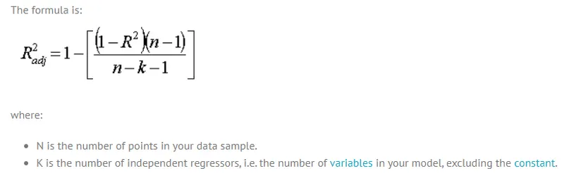
The adjusted R^2 will penalize you for adding independent variables (K in the equation) that do not fit the model. Inregression analysis, it can be tempting to add more variables to the data as you think. The adjusted R^2 will compensate for this by that penalizing you for those extra variables.

Both R^2 and the adjusted R^2 give you an idea of how many data points fall within the line of the regression equation. However, there is one main difference between them, R^2 assumes that every single variable explains the variation in the dependent variable. The adjusted R² tells you the percentage of variation explained by only the independent variables that actually affect the dependent variable.