Supervised Learning - Prediction Week 3 Challenge

Ans 1: Code to perform gradient descent using mean square error as loss function and predicting the output. The data used is age of person and the average money spent by them on medical expenses per month.

# Importing the required library
import numpy as np

# Function to perform Gradient descent
def gradient_descent(x,y):
    m_curr=b_curr=0
    learning_rate=0.0001
    previous=None
    i=0
      
    while True:
        y_predicted = m_curr*x + b_curr
        error = (1/n)*sum([val**2 for val in (y-y_predicted)])
        if previous is not None and abs(previous-error)<0.000000000001:
            break
         
        md = -(2/n)*sum(x*(y-y_predicted))
        bd = -(2/n)*sum(y-y_predicted)
        m_curr = m_curr-learning_rate*md
        b_curr = b_curr-learning_rate*bd
        previous=error
        i=i+1
    print("number of iterations :",i)     
    return m_curr,b_curr 

# Function to predict the output
def predict(x1):
    x=np.array([15,20,25,37,40,45,48,50,55,61 ])  #age of persons
    y=np.array([100,135,135,150,250,270,290,360,375,400])#money spent on health/month 
    m,b =gradient_descent(x,y)
    y = m*x1 + b
    return m,b,y

#lets predict and print the output at input of 65(age)
m,b,y1=predict(65)
print("slope :",m)
print("Intercept :",b)
print("The predicted :",y1)                         

Ans 2: L1 and L2 both are used to minimize overfitting of data by adding some penalty in the loss function.

In L1 method we add λ*∑|wj| in the loss function , where wj is the value of weight and λ is a constant which can be tuned.

In L2 method we add λ*∑(wj)^2 in the loss function.

The main difference between L1 and L2 is that L1 tries to estimate median of the data, while L2 tries to estimate mean of the data to avoid overfitting. L1 adds the penalty term in cost function by adding the absolute value of weight(Wj) parameters, while L2 adds the squared value of weights(Wj) in the cost function.

While taking derivative of the cost function, in L1 it will estimate around the median of the data. where as in L2, while calculating the loss function in the gradient calculation step, the loss function tries to minimize the loss by subtracting it from the average of the data distribution.

Ans 3: different loss functions for regression are:-

(2.1) Mean square error(MSE) - it is the most commonly used loss function in regression. MSE is the sum of squared distances between our target variable and predicted values.

MSE= (1/n)*∑(y - yp)^2

(2.2) Mean absolute error(MAE) - MAE is the sum of absolute differences between our target and predicted variables.

MAE= (1/n)*∑|y - yp|

MAE is more robust to outliers, but its derivatives are not continuous, making it inefficient to find the solution. MSE is more sensitive to outliers, but gives a more stable and closed form solution.

(2.3) Huber loss - huber loss is less sensitive to outliers in data than the squared error loss. It’s also differentiable at 0. It’s basically absolute error, which becomes quadratic when error is small. How small that error has to be, to make it quadratic depends on a hyperparameter, 𝛿(delta), which can be tuned. Huber loss approaches MSE when 𝛿 ~ 0 and MAE when 𝛿 ~ ∞ (large numbers.)

L(y,f(x)) = 1/2(y - f(x))^2 if |y-f(x)|≤ 𝛿

= 𝛿|y - f(x)| - (1/2)*𝛿 otherwise

(2.4) Log-cosh loss - Log-cosh is the logarithm of the hyperbolic cosine of the prediction error. it is smoother than MSE.

L(y,yp) = ∑ log(cosh(yp - y))

log(cosh(x)) is approximately equal to (x^2)/2 for small x and abs(x) - log(2) for large x.It means that logcosh works mostly like the mean squared error, but will not be so strongly affected by the occasional wildly income of prediction. It has the advantages of huber loss, and it is twice differentiable everywhere.

Ans 4: Learning rate decides the speed by which we move to minimum error point from some starting point.

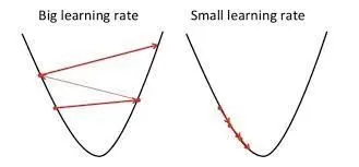
If the learning rate is very high then we may surpass the minimun point and never arrive at it ,and if the learning rate is too low then it takes a lot of time to reach at minimum point ,so a optimum value of learning rate should be chosen.

Ans 5: Steps to evaluate linear regression :-

• Divide the data into training and test data sets. Its important because the model will be build on training data set and its performance will be checked on test data set.
• Chosing the appropriate loss function, which may include L1 and L2 regularization.
• minimizing the value of loss function by differentiating it with respect to slope(m) and intercept(b) of the linear equation(y = m*x + b).
• calculating the value m and b at which loss is minimum.
• putting back the value of m and b in equation y = m*x + b ,now the model is ready for prediction.
• The model efficancy can be calculated by calculating the coefficient of determination(R^2) to see its accuracy.

Ans 6: R^2 or coefficient of determination represents the proportion of varience(of y) that has been explained by the independent variable in the model. Basically it tells how accurate your fit is.

R^2 = 1 - (MSE/Mean variation in y)

= 1 - ((1/n)*∑(y - yp)^2)/((1/n)*∑(y - yavg)) where yp is the predicted value and yavg is the average value of y.

one limitaion of R^2 is that it increases by adding independent variables to the model which is misleading since some added variables might be usefull with minimal significance.

so, Adjusted R^2 overcomes this issue by adding a penalty if we make an attempt to add aindependent variables that does not improve the model.

Adjusted R^2 = 1 - [(1-R^2)*(n-1)/(n-k-1)] where k is the number of independent variables and n is the number of samples.

If useless predictors are added then Adjusted R^2 decreases

If usefull predictors are added then Adjusted R^2 increases