Supervised Learning - Prediction Week 3 Challenge

1)

import numpy as np

# Define the data
X = np.array([1, 2, 3, 4, 5])
y = np.array([5, 7, 9, 11, 13])

# Define the initial values of the parameters
m = 0
b = 0

# Define the learning rate and the number of iterations
learning_rate = 0.01
iterations = 1000

# Define the MSE loss function
def mse_loss(y_true, y_pred):
    return ((y_true - y_pred) ** 2).mean()

# Define the gradient descent function
def gradient_descent(X, y, m, b, learning_rate, iterations):
    N = len(X)
    for i in range(iterations):
        y_pred = m * X + b
        d_m = (-2/N) * sum(X * (y - y_pred))
        d_b = (-2/N) * sum(y - y_pred)
        m = m - learning_rate * d_m
        b = b - learning_rate * d_b
        if i % 100 == 0:
            print(f"Iteration {i}, loss: {mse_loss(y, y_pred)}")
    return m, b

# Run the gradient descent function
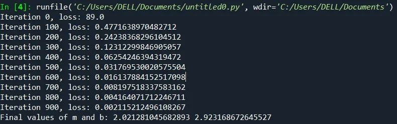
m, b = gradient_descent(X, y, m, b, learning_rate, iterations)

# Print the final values of the parameters
print("Final values of m and b:", m, b)

2)

The L1 is also know as Lasso regression.Lasso is an acronym for least absolute shrinkage and selection operator, and lasso regression adds the “absolute value of magnitude” of the coefficient as a penalty term to the loss function.

L2 is known as Ridge regression.Ridge regression adds the “squared magnitude” of the coefficient as the penalty term to the loss function.

The main difference between the two methods is that L1 regularization tends to produce sparse models, where many of the model parameters are set to zero. This is because the L1 penalty encourages many of the parameters to be exactly zero. In contrast, L2 regularization tends to produce models where all of the model parameters are non-zero, but small. This is because the L2 penalty encourages the model parameters to be small, but does not force any of them to be exactly zero.

3)

The different loss functions are as follows:

• Mean Squared Error/L2 loss
• Mean Absolute Error/L1 loss
• Root Mean Squared Error
• Mean bias error
• Huber loss

Similarly for Binary classification error function,

• Binary-cross entropy loss
• Hinge loss
• Squared hinge loss

Multinomial Classification loss function:

• categorical cross-entropy loss
• KL divergence

4)

The learning rate controls how quickly the model is adapted to the problem. Smaller learning rates require more training training epochs given the smaller changes made to the weights each update, whereas larger learning rates result in rapid changes and require fewer training epochs.

A learning rate that is too large can cause the model to converge too quickly to a suboptimal solution, whereas a learning rate that is too small can cause the process to get stuck.

5)

To evaluate Linear regression we choose any of the following:

1. R Square/Adjusted R Square
2. Mean Square Error(MSE)/Root Mean Square Error(RMSE)
3. Mean Absolute Error(MAE)
4. R-squared (R2)
5. Adjusted R-squared
6. Residual plots
7. Cross-validation

6)

Multiple R squared is simply a measure of R squared for models that have multiple predictor variables. Therefore it measures the amount of variation in the response variable that can be explained by the predictor variables. The fundamental point is that when you add predictors to your model, the multiple Rsquared will always increase, as a predictor will always explain some portion of the variance.

Adjusted Rsquared controls against this increase, and adds penalties for the number of predictors in the model. Therefore it shows a balance between the most parsimonious model, and the best fitting model. Generally, if you have a large difference between your multiple and your adjusted Rsquared that indicates you may have overfit your model.