Supervised Learning - Prediction Week 3 Challenge

1. Perform Gradient Descent in Python with any loss function

The data set used is as follows:

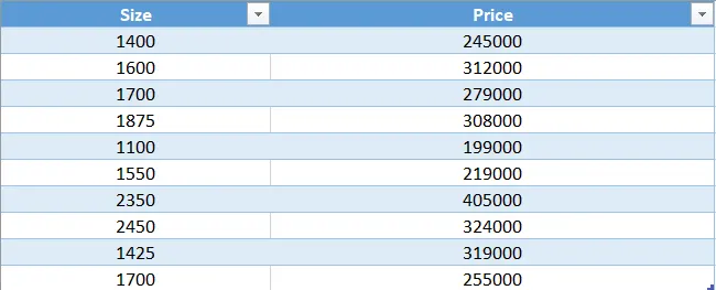
Here an effort is made to use regression analysis for curve fitting. And, the loss function used to fit the curve is Mean square error.

`J=(1/n) sum(y(i)-(mx(i)+b))^2`

x(i) is the input

m and b are slope and intercept.

y(i) is the actual value and mx(i)+b is the predicted value.

Now we need to determine the values of m and b such that the J is minimized.

Differentiating the loss function J w.r.t to m and b, we get

`(dJ)/(dm) = (2/n)sum-x(i)(y(i)-(mx(i)+b))`

`(dJ)/(db) = (2/n)sum-(y(i)-(mx(i)+b))`

m and b values are then optimized.

Then we introduce the learning rate (LR) to move the values of m and b towards minimizing J.

`m=m-LR*(dJ)/(dm)`

`b=b-LR*(dJ)/(db)`

As the data in both the columns are vary in thousands in one column to 100 thousands in other column. In order for optimization to run faster we normalise the data as below.

`x_s(i)=(x(i)-min(x))/(max(x)-min(x))`

`y_s(i)=(y(i)-min(y))/(max(y)-min(y))`

Then the data is converted as below:

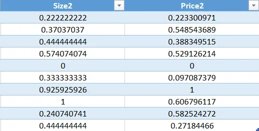
As the data is in CSV format, at first it is read in python then normalization is applied by using the following code:

import numpy as np 
import matplotlib.pyplot as plt 
from statistics import mean 
import pandas as pd

df = pd.read_csv(r'F:\AI ML skill lync\week 3\data1.csv')
Size=df['Size']
Price = df['Price']

n = len(Size)

# Normalization of data
Size_S = []
Price_S = []
for i in range(0,n):
	Size_S.append((Size[i]-min(Size))/(max(Size)-min(Size)))
	Price_S.append((Price[i]-min(Price))/(max(Price)-min(Price)))

Then we initialize the parameters to start our algorithm

#intialising the parameters
m = 0
b = 0
J = 9e9 #cost function
tol = 1e-4 # error tolerance

#learning rate
LR = 0.01

iter = 1 

Main body of the code where the gradient descent is formulated, after every iteration the loss functions, slope and intercept are updated with in the while loop. Moreover, loop breaker is used if the iterations reach 1e4 using break.

while(J>tol):
	j_arr = []
	d_m = []
	d_b = []

	for i in range(0,n):
		j_arr.append(pow((Price_S[i]-m*Size_S[i]-b),2))
		d_m.append(-Size_S[i]*(Price_S[i]-m*Size_S[i]-b))
		d_b.append(-(Price_S[i]-m*Size_S[i]-b))

	# updating the values

	J = 1/n * sum(j_arr)
	m=m-LR*(2/n)*sum(d_m)
	b=b-LR*(2/n)*sum(d_b)

	print("\n Number of Iterations: ",str(iter) + "		Error = ", str(J))
	iter = iter+1

	#iteration breaker
	if iter>1e5:
		print('reached iterations limit')
		break

Once the convergence tolerance or iterations limit is reached. We calculate the slope and intercept for our data by using the following formula:

As the data normally standardize, the equation is as follows:

`y_s = mx_s+b`

we need to replace y_s and x_s into y and x.

`x_s(i)=(x(i)-min(x))/(max(x)-min(x))`

`y_s(i)=(y(i)-min(y))/(max(y)-min(y))`

Putting these equations in the above slope intercept line equation we get:

`(y(i)-min(y))/(max(y)-min(y))=m(x(i)-min(x))/(max(x)-min(x))+b`

converting this equation to slope intercept form, we get m and b for old data (non-normalized) represented as m_NS and b_NS.

`m_(NS) = m*(max(y)-min(y))/(max(x)-min(x))`

`b_(NS) = b*(max(y)-min(y))-m*min(x)*(max(y)-min(y))/(max(x)-min(x))+min(y)`

Slope and intercept for actual data are determined and values of function are predicted using slope and intercept.

# Reformating  slope and intercept for actual data
m_NS = m*(max(Price)-min(Price))/(max(Size)-min(Size))
b_NS = b*(max(Price)-min(Price))-m*min(Size)*(max(Price)-min(Price))/(max(Size)-min(Size))+min(Price)

Price_p = []
for i in range(0,n):
	Price_p.append(m_NS*Size[i]+b_NS)

Calculation of R^2:

It is determined using the sum of squared differences of predicted values and mean over sum of squared differences of actual values and mean.

#Calculation of R^2
mean_price = mean(Price)
# calculation of sum of squared differences SST
SST = []
for i in range (0,n):
	SST.append((Price[i]-mean_price)**2)
SST_val = sum(SST)

# calculation of sum of squared differences of predicted values SSR
mean_price_p = mean(Price_p)
SSR = []
for i in range (0,n):
	SSR.append((Price_p[i]-mean_price_p)**2)
SSR_val = sum(SSR)

R_square = SSR_val/SST_val

Visualization is done by using the following code:

# function for truncating the decimals to 3 places
def truncate(n, decimals=0):
    multiplier = 10 ** decimals
    return int(n * multiplier) / multiplier

#visualization
plt.scatter(Size,Price,label = "Actual Price")
plt.plot(Size,Price_p,'-r',label = "Predicted Price")
plt.xlabel('Size (Sq.ft)')
plt.ylabel('Price ($)')
plt.title('Linear Regression of Housing Price')
plt.legend(loc='upper left',fontsize=14)
plt.text(2200, 2.3e5, r'R$^2$ = '+str(truncate(R_square,3)))
plt.text(2090, 2.1e5, r'y='+str(truncate(m_NS,3))+r'x+'+str(truncate(b_NS,3)))
plt.show()

Output:

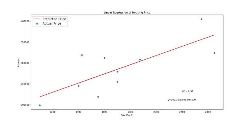
Validation:

from sklearn import linear_model

reg1 = linear_model.LinearRegression()
reg2 = linear_model.LinearRegression()

reg1.fit(df[["Size"]],df[["Price"]])

reg2.fit(np.array(Size_S).reshape(-1, 1),np.array(Price_S).reshape(-1, 1))

print("The value of m for standardize data using code: ", str(m))
print("The value of m for data using code: ", str(m_NS))
print("The value of m for standardize data using library: ", str(reg2.coef_))
print("The value of m for data using library: ", str(reg1.coef_))

print("The value of b for standardize data using code: ", str(b))
print("The value of b for data using code: ", str(b_NS))
print("The value of b for standardize data using library: ", str(reg2.intercept_))
print("The value of b for data using library: ", str(reg1.intercept_))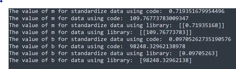

Thus, the results obtained are in agreement with the ones obtained by sklearn library.

Difference between L1 & L2 Gradient descent method

Mean Absollute Error, L1-(MAE) is another loss function used for regression models. MAE is the sum of absolute differences between our target and predicted variables. So it measures the average magnitude of errors in a set of predictions, without considering their directions. (If we consider directions also, that would be called Mean Bias Error (MBE), which is a sum of residuals/errors). The range is also 0 to ∞.

`MAE = (1/n)sum_(i=1)^n abs(y_i-y_i^p`

Mean Squared Error, L2-(MSE) is the most commonly used regression loss function. MSE is the sum of squared distances between our target variable and predicted values.

`MSE = (1/n)sum_(i=1)^n(y_i-y_i^p)^2`

Since MSE squares the error (y — y_predicted = e), the value of error (e) increases a lot if e > 1. If we have an outlier in our data, the value of e will be high and e² will be >> |e|. This will make the model with MSE loss give more weight to outliers than a model with MAE loss.

What are the different loss functions for regression

The different loss functions used are as follows:

1. Mean Square Error
2. Mean Absolute Error
3. Root Mean Square Error
4. Huber loss
5. Log-cosh loss
6. Quantile loss (this is used to find range of predictions)

What is the importance of learning rate

The learning rate is a configurable hyperparameter used in the training of neural networks that has a small positive value, often in the range between 0.0 and 1.0.

The learning rate controls how quickly the model is adapted to the problem. Smaller learning rates require more training epochs given the smaller changes made to the weights each update, whereas larger learning rates result in rapid changes and require fewer training epochs.

A learning rate that is too large can cause the model to converge too quickly to a suboptimal solution, whereas a learning rate that is too small can cause the process to get stuck.

The challenge of training deep learning neural networks involves carefully selecting the learning rate. It may be the most important hyperparameter for the model.

How to evaluate linear regression

Linear regression can be evaluated by determining how good the fit is i.e., the error between the predicted value and the data set.

In statistics, the coefficient of determination, denoted R² or r² and pronounced "R squared", is the proportion of the variance in the dependent variable that is predictable from the independent variable(s).

For the data it can be found as below:

`R^2 =(SSR)/(SST)`

The sum of squares total, denoted SST, is the squared differences between the observed dependent variable and its mean.

`SST =sum_(i=1)^n(y_i-bar y)^2`

The second term is the sum of squares due to regression, or SSR. It is the sum of the differences between the predicted value and the mean of the dependent variable.

`SSR =sum_(i=1)^n(y_i^P-bar y)^2`

What is the difference between multiple and adjusted coefficient of determination

When the dependent variable depends on only one independent variable then it is known as the linear coefficient of determination, but when it depends on multiple independent variables then it is multiple coefficient of determination.

The adjusted coefficient of determination is the method in which the parameters which do not contribute towards the predicted value are ignored. These parameters are called insignificant independent variables.

Adding new variables to the system will affect the R-squared value and the adjusted R-Squared discards the infinitesimly small increments and only considers the parameters which contribute to the output in a significant way.

`R_(adj)^2 = 1- ((1-R^2)*(n-1))/(n-k-1)`

n = number of data points

k = number of independent points

Case 1: If added variables are insignificant, that means k will increase with little or no effect on `R^2`, hence `R^2_(adj)` will decrease.

Case 2: If added variables are insignificant, that means k will increase with a significant increase on `R^2`, hence `R^2_(adj)` will increase.