Supervised Learning - Prediction Week 3 Challenge

1.Perform Gradient Descent in Python with any loss function

- Code for the Gradient Descent is

 import numpy as np
 def gradient_descent(x,y):
     m_curr = b_curr = 0
     iterations=1000
     n = len(x)
     learning_rate = 0.08

     for i in range(iterations):
          y_predicted = m_curr * x + b_curr
          cost = (1/n)* sum([val ** 2 for val in (y - y_predicted)])
          md = -(2/n)* sum(x* (y-y_predicted))
          bd = -(2/n) * sum((y - y_predicted))
          m_curr= m_curr - learning_rate * md
          b_curr= b_curr - learning_rate * bd
          print ("m {}, b {}, cost {}, iteration {}".format(m_curr,b_curr,cost, i))

 x=np.array([1,2,3,4,5])
 y=np.array([5,7,9,11,13])

 gradient_descent(x,y)
 
 

x	y	a=x-x_	b=y-y_	(x-x_)^2	a*b
1	5	-2	-4	4	8
2	7	-1	-2	1	2
3	9	0	0	0	0
4	11	1	2	1	2
5	13	2	4	4	8

Mean(x_)=3

Mean(y_)=9

slope m = (a*b)/(x-x_)^2=20/10=2, m=2

Equation of the slope is : y_=(m)(x_)+b

y_=9, x_=3, m=3

b=3 which is the y-intercept

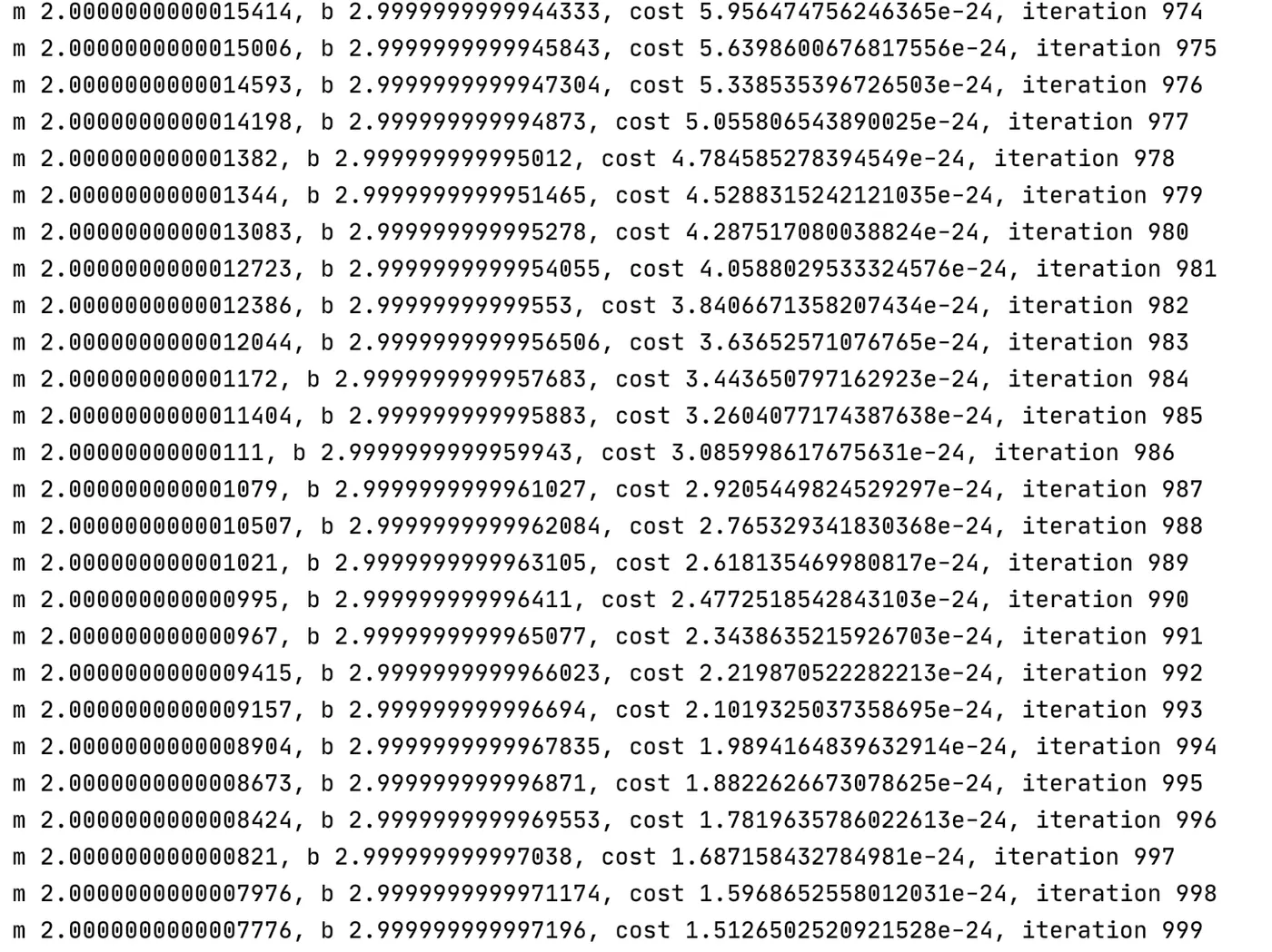
Now from the output of the code, we have 'm' and 'b' values to be equal to 2.0000000000007775 and 2.9999999999997176 which is almost equal to the calculated value of 2 and 3 for the slope and intercept.

And by finding the co-efficients of the function parameters we are able to keep the cost low or rather minimise the cost as far as possible.

2.Difference between L1 & L2 Gradient descent method

- Mean Absolute Error (L1) = (1/n) ∑l Y(actual) - Y(predicted) l

Mean Square Error (L2) = (1/n) ∑[Y(actual) - Y(predicted)]^2

- In the L1 formula we have to take the absolute value to the cost function and in the L2 formula we square the cost funtion.

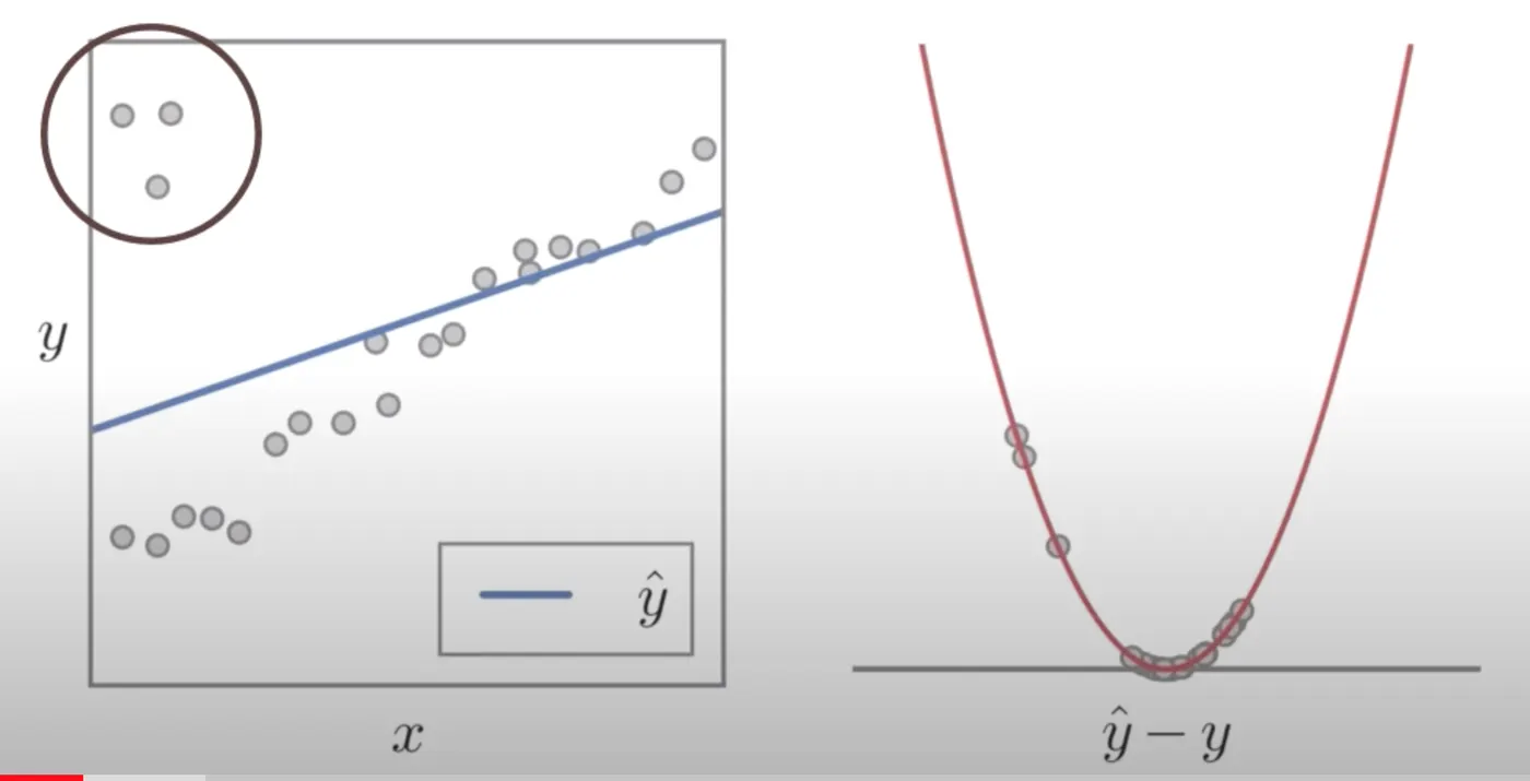
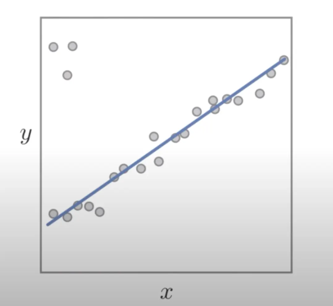
- The main difference between L1 and L2 regularization is that L1 tries to give us the median of the data, whereas L2 tries to gibe us the mean us the mean of the data.

-

L2 L1

L2 can lead to poor predictions as it is not affected by outliers as the model won't respond properly since it is affeceted by the square term which scales the errors by the outliers in the loss function, whereas L1 is not affected by outliers from time time to time due to the absolute difference.

3.What are the different loss functions for regression

The different types of regressions are

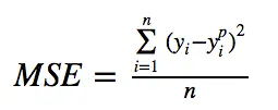
- Mean Square Error(MSE,L2): Is the most commonly used regression loss function. MSE is the sum of squared distances between our target variable and predicted values.

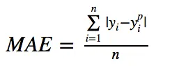
- Mean absolute Error(L1):MAE is the sum of absolute differences between our target and predicted variables.

- Huber loss/Smooth Mean Absolute Error: Huber loss is less sensitive to outliers in data than the squared error loss. It’s also differentiable at 0. It’s basically absolute error, which becomes quadratic when error is small.

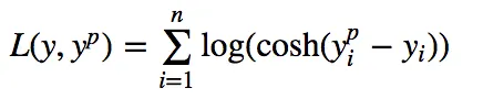
- Log Cosh Loss: Log-cosh is another function used in regression tasks that’s smoother than L2. Log-cosh is the logarithm of the hyperbolic cosine of the prediction error.

- Quantile Loss:Quantile Loss is useful when we are interested in predicting an interval instead of only point predictions. Prediction interval from least square regression is based on an assumption that residuals (y — y_hat) have constant variance across values of independent variables.

4.What is the importance of learning rate

-Learning rate is a tuning parameter in an optimization algorithm that determines the step size at each iteration while moving toward a minimum of a loss function.

-A smaller learning rate may allow the model to learn a more optimal or even globally optimal set of weights but may take significantly longer to train.

-Learning rate gives the rate of speed where the gradient moves during gradient descent. Setting it too high would make your path instable, too low would make convergence slow.

-There are multiple ways to select a good starting point for the learning rate. One approach is to try a few different values and see which one gives you the best loss without sacrificing speed of training. We might start with a large value like 0.1, then try exponentially lower values: 0.01, 0.001, etc.

5.How to evaluate linear regression

- Linear regression is evaluated by the R Square/Adjusted R Square.

- Regression analysis is a form of predictive modelling technique which investigates the relationships between dependant and independant variables

- In a simple linear regression we are interested in the equation of the slope which is y = (m)(x)+b where 'm' is the slope and 'b' is the y-intercept adn we are interested to find the co-relation between the x(Independant variable) and y(Dependant variable)

- To evaluate the code in python we use the following code,

from sklearn import linear_model

reg=linear_model.LinearRegression()

sklearn is the heart of machine learning. Linear regression is in-built in "from sklearn import linear_model"

6.What is the difference between multiple and adjusted coefficient of determination

-R-squared is a statistical measure of how close the data are to the fitted regression line. It is also known as the coefficient of determination, or the coefficient of multiple determination for multiple regression.

-Multiple linear regression is a statistical technique that uses several variables to predict the outcome of a different variable. The goal of multiple regression is to model the linear relationship between the independent variables and the dependent variable.

- Adjusted R-squared is a modified version of R-squared that has been adjusted for the number of predictors in the model. The adjusted R-squared increases only if the new value improves the model more than would be expected by chance. It decreases when a predictor improves the model by less than expected by chance