Supervised Learning - Classification Week 8 Challenge

First all the required libraries are imported and the dataset is loaded.

import numpy as np
import pandas as pd
import matplotlib.pyplot as plt
from sklearn.datasets import load_iris
from sklearn.metrics import confusion_matrix
from sklearn.metrics import classification_report
from sklearn.model_selection import train_test_split
import seaborn as sns

from sklearn.cluster import DBSCAN
from collections import Counter

Data is read on the compiler.

df = pd.read_csv('faults.csv')
df.head() # to check the top 5 rows of data
len(df.columns) # to find the overview of features and targets

The last 7 columns are the defects and are one-hot encoded.

Lets segregate the features and targets

y=df.iloc[:,27:34];
X=df.iloc[:,0:27];

Lets normalize the data as every feature has different scale.

from sklearn.preprocessing import MinMaxScaler

sc = MinMaxScaler(feature_range =(0,1))

X_std = pd.DataFrame(sc.fit_transform(X), columns = X.columns)
print(X_std.shape)
X_std.boxplot(figsize = (12.8,8), rot = 90)
plt.boxplot
plt.show()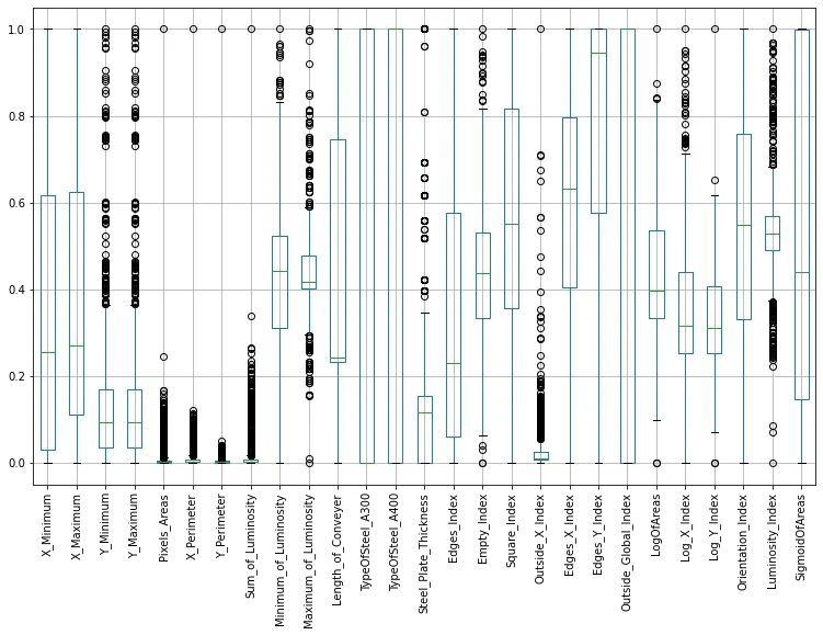

Lets check if there are any null records.

#check missing values
plt.figure(figsize=(12,4))
sns.heatmap(df.isnull(),cbar=False,cmap='Wistia',yticklabels=False)
plt.title('Missing value in the dataset');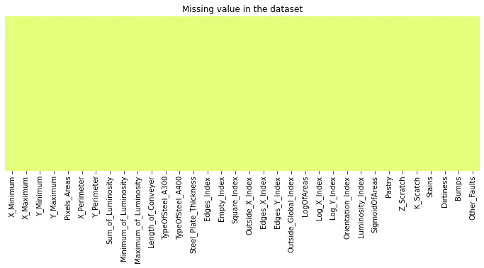

There is no null data.

Lets convert the target columns in to single target column using the categorical values of defects.

df = pd.read_csv('faults.csv')
targets = df.iloc[:, 27:]
df.drop(targets.columns, axis=1, inplace=True)
df['Target'] = targets.idxmax(1)

df['Target']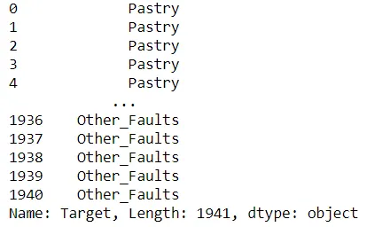

Lets look at the count of defects.

target_counts= df['Target'].value_counts()

fig, ax = plt.subplots(1, 2, figsize=(15,7))
target_counts_barplot = sns.barplot(x = target_counts.index,y = target_counts.values, ax = ax[0])
target_counts_barplot.set_ylabel('Number of classes in the dataset')

target_counts.plot.pie(autopct="%1.1f%%", ax=ax[1])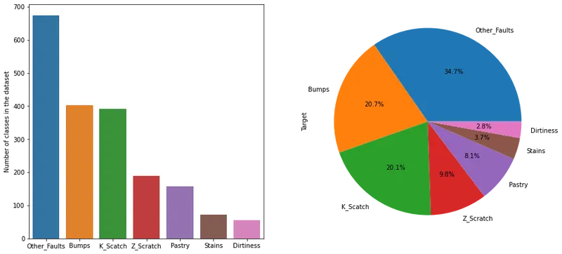

Lets look at the correlation between the input data.

plt.figure(figsize=(20,15))
sns.heatmap(df.corr(), cmap='hsv')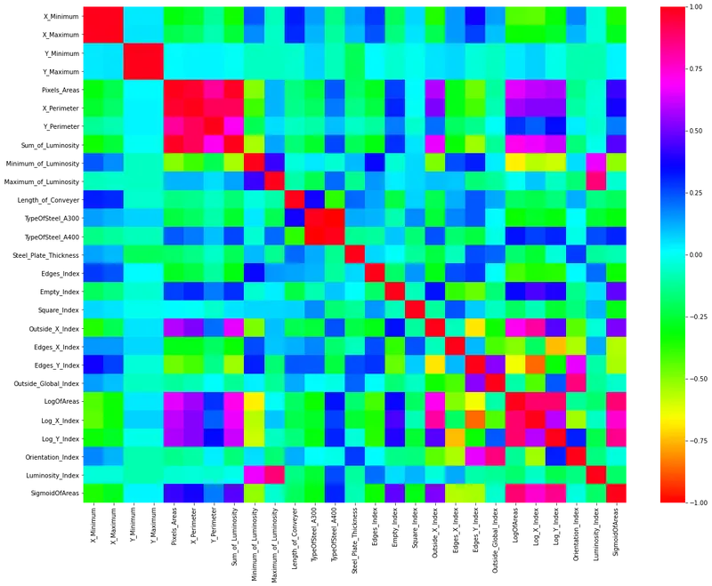

Lets add one more column to our data frame to have nominal values of our 'target' in 'Target_Code' column.

df['Target'] = pd.Categorical(df['Target'])
df['Target_Code'] = df.Target.cat.codes

Let us look at the outliers of data.

plt.figure(figsize=(8,5))
sns.boxplot(x=y, y=X_std['X_Maximum'])

There are many outliers, so we can use 'DBSCAN' method to remove few outliers by using clusters.

The input to the 'DBSCAN' method are radius of neighbourhood and cluster size, to eliminate those outliers.

I wrote a small code to find the optimum value of radius to eliminate the 5% of data.

eps_r = 0.1
while eps_r < 10:
    dbscan_model = DBSCAN(eps=eps_r, min_samples=7).fit(X_std) 
    
    if Counter(dbscan_model.labels_)[-1] < 0.05*len(X_std):
        print('The neighbourhood distance considered for removal of less than 5% outliers is: {}'.format(eps_r))
        break
        
    eps_r = eps_r + 0.1

The neighbourhood distance considered for removal of less than 5% outliers is: 0.7

Lets check how many values are eliminated from our dataframe.

dbscan_model = DBSCAN(eps=eps_r, min_samples=7).fit(X_std)
print(Counter(dbscan_model.labels_)[-1])

38

Lets eliminate the outliers

outliers = X_std[dbscan_model.labels_ == -1]
outliers.shape

X_std.drop(outliers.index, axis=0, inplace=True)
y.drop(outliers.index, axis=0, inplace=True)

Lets split the training and testing dataset.

# Splitting the dataset into the Training set and Test set
X_train, X_test, y_train, y_test = train_test_split(X_std, y, train_size = 0.9, random_state = 0)

We will be training our data on 5 different models and select the one with best accuracy.

1. Logistic Regression
2. Decision Tree
3. Random Forest
4. Support Vector Machine
5. K-Nearest Neighbours

All the data models will be built on default hyperparameters.

Logistic Regression

# LogisticRegression
from sklearn.linear_model import LogisticRegression
LogReg = LogisticRegression()
LogReg.fit(X_train, y_train)

y_pred_LogReg = LogReg.predict(X_test)

# Summary of the predictions made by the classifier
print(classification_report(y_test, y_pred_LogReg))
print(confusion_matrix(y_test, y_pred_LogReg))
# Accuracy score
from sklearn.metrics import accuracy_score
print('accuracy is',accuracy_score(y_pred_LogReg,y_test))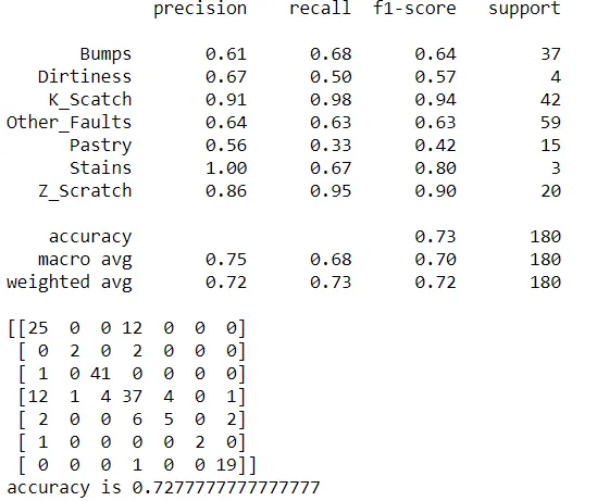

#Plotting the confusion matrix.

from sklearn.metrics import confusion_matrix

cm = confusion_matrix(y_test, y_pred_LogReg)

print(cm)
plt.figure(figsize=(10,7))
categories = np.unique(y)
df_cm = pd.DataFrame(cm, index = [i for i in categories], columns = [i for i in categories])
sns.heatmap(df_cm,annot=True,cmap='Reds')
plt.xlabel("Predicted")
plt.ylabel("Actual")
plt.show()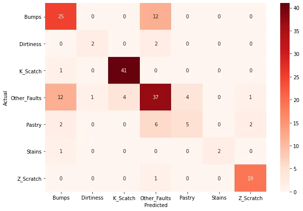

Decision Tree

from sklearn.tree import DecisionTreeClassifier

DTC = DecisionTreeClassifier()

DTC.fit(X_train, y_train)

y_pred_DTC = DTC.predict(X_test)

# Summary of the predictions made by the classifier
print(classification_report(y_test, y_pred_DTC))
print(confusion_matrix(y_test, y_pred_DTC))
# Accuracy score
from sklearn.metrics import accuracy_score
print('accuracy is',accuracy_score(y_pred_DTC,y_test))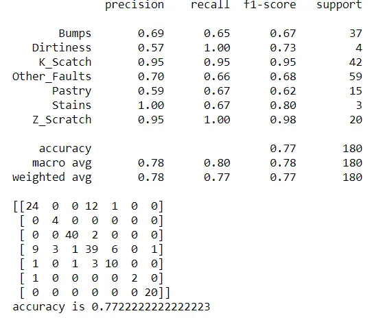

#Plotting the confusion matrix.

from sklearn.metrics import confusion_matrix

cm = confusion_matrix(y_test, y_pred_DTC)

print(cm)
plt.figure(figsize=(10,7))
categories = np.unique(y)
df_cm = pd.DataFrame(cm, index = [i for i in categories], columns = [i for i in categories])
sns.heatmap(df_cm,annot=True,cmap='Reds')
plt.xlabel("Predicted")
plt.ylabel("Actual")
plt.show()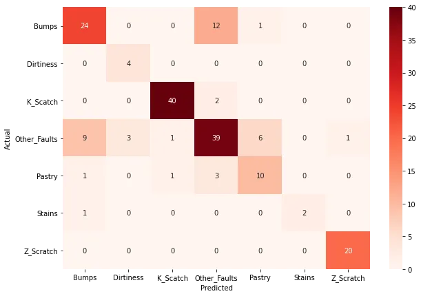

Support Vector Machine:

# Support Vector Machine's 
from sklearn.svm import SVC

SVM_C = SVC(kernel='linear')
SVM_C.fit(X_train, y_train)

y_pred_svm = SVM_C.predict(X_test)

# Summary of the predictions made by the classifier
print(classification_report(y_test, y_pred_svm))
print(confusion_matrix(y_test, y_pred_svm))
# Accuracy score
from sklearn.metrics import accuracy_score
print('accuracy is',accuracy_score(y_pred_svm,y_test))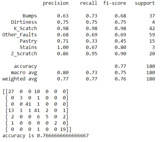

#Plotting the confusion matrix.

from sklearn.metrics import confusion_matrix

cm = confusion_matrix(y_test, y_pred_svm)

print(cm)
plt.figure(figsize=(10,7))
categories = np.unique(y)
df_cm = pd.DataFrame(cm, index = [i for i in categories], columns = [i for i in categories])
sns.heatmap(df_cm,annot=True,cmap='Reds')
plt.xlabel("Predicted")
plt.ylabel("Actual")
plt.show()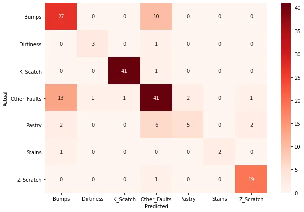

Random Forest Classifier

# Random Forest
from sklearn.ensemble import RandomForestClassifier

RFC= RandomForestClassifier()
RFC.fit(X_train, y_train)

y_pred_RFC = RFC.predict(X_test)

# Summary of the predictions made by the classifier
print(classification_report(y_test, y_pred_RFC))
print(confusion_matrix(y_test, y_pred_RFC))
# Accuracy score
from sklearn.metrics import accuracy_score
print('accuracy is',accuracy_score(y_pred_RFC,y_test))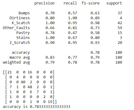

#Plotting the confusion matrix.

from sklearn.metrics import confusion_matrix

cm = confusion_matrix(y_test, y_pred_RFC)

print(cm)
plt.figure(figsize=(10,7))
categories = np.unique(y)
df_cm = pd.DataFrame(cm, index = [i for i in categories], columns = [i for i in categories])
sns.heatmap(df_cm,annot=True,cmap='Reds')
plt.xlabel("Predicted")
plt.ylabel("Actual")
plt.show()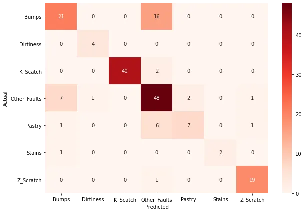

K-Nearest Neighbor Classifier:

from sklearn.neighbors import KNeighborsClassifier
KNN=KNeighborsClassifier()
KNN.fit(X_train, y_train)

y_pred_KNN = KNN.predict(X_test)

# Summary of the predictions made by the classifier
print(classification_report(y_test, y_pred_KNN))
print(confusion_matrix(y_test, y_pred_KNN))
# Accuracy score
from sklearn.metrics import accuracy_score
print('accuracy is',accuracy_score(y_pred_KNN,y_test))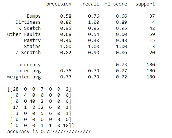

#Plotting the confusion matrix.

from sklearn.metrics import confusion_matrix

cm = confusion_matrix(y_test, y_pred_KNN)

print(cm)
plt.figure(figsize=(10,7))
categories = np.unique(y)
df_cm = pd.DataFrame(cm, index = [i for i in categories], columns = [i for i in categories])
sns.heatmap(df_cm,annot=True,cmap='Reds')
plt.xlabel("Predicted")
plt.ylabel("Actual")
plt.show()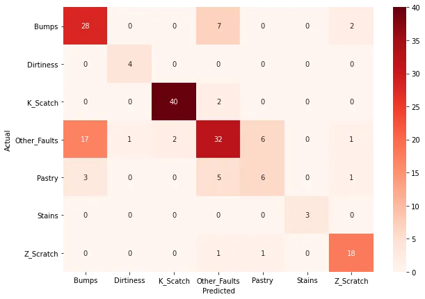

Let us compare the accuracy of all the classifiers.

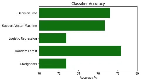
It can be observed that of all the classifiers the accuracy of the Random Forest Model is higher.

Pros of KNN:

1. Intutive and simple
2. No assumptions
3. No Training Step
4. It evolves constantly
5. Very easy to implement for multi-class problem
6. Can be used for both classification and regression

Cons of KNN:

1. Becomes slow as the dataset grows
2. Curse of dimensionality
3. Need of homogeneous features
4. Optimal number of neighbours required
5. Inbalanced data causes problems
6. Outlier sensitivity