Supervised Learning - Classification Week 8 Challenge

Question 2.

Advantages of KNN

1. No Training Period: KNN is called Lazy Learner (Instance based learning). It does not learn anything in the training period. It does not derive any discriminative function from the training data. In other words, there is no training period for it. It stores the training dataset and learns from it only at the time of making real time predictions. This makes the KNN algorithm much faster than other algorithms that require training e.g. SVM, Linear Regression etc.

2. Since the KNN algorithm requires no training before making predictions, new data can be added seamlessly which will not impact the accuracy of the algorithm.

3. KNN is very easy to implement. There are only two parameters required to implement KNN i.e. the value of K and the distance function (e.g. Euclidean or Manhattan etc.)

Disadvantages of KNN

1. Does not work well with large dataset: In large datasets, the cost of calculating the distance between the new point and each existing points is huge which degrades the performance of the algorithm.

2. Does not work well with high dimensions: The KNN algorithm doesn't work well with high dimensional data because with large number of dimensions, it becomes difficult for the algorithm to calculate the distance in each dimension.

3. Need feature scaling: We need to do feature scaling (standardization and normalization) before applying KNN algorithm to any dataset. If we don't do so, KNN may generate wrong predictions.

4. Sensitive to noisy data, missing values and outliers: KNN is sensitive to noise in the dataset. We need to manually impute missing values and remove outliers.

Question 1.

KNN: K-Nearest Neighbors is a supervised machine learning algorithm that classifies a data point based on how its neighbors are classified. It classifies new cases based on feature similarity measures.

KNN algorithm

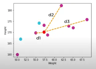
k in the KNN algorithm is a parameter that refers to the number of nearest neighbors to include in the majority voting process. It is important to choose the right value of k in order to attain high model accuracy and this is achieved by parameter tuning.

KNN is used for data that is labeled, small in size, and noise-free.

KNN algorithm calculates the distance between two points using the Euclidean formula.

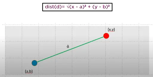
It'll calculate the distance between the unknown data point and all the points in the dataset, and based on the distance value, it'll classify the data point.

Pros:

• It is a simple Machine Learning algorithm and easy to understand.
• kNN can be used for classification and regression.
• It can be used for multi-class problem.
• It provides a variety of distance criteria to choose from: Euclidean Distance Hamming Distance Manhattan Distance Minkowski Distance

Cons:

• It is difficult to choose the optimal number of neighbors to be consider while classifying the new data entry.
• K-NN inherently has no capability of dealing with missing value problem.
• k Nearest Neighbor has calculate the proximity between each neighbors for every single value in the dataset. For large daasets its computation cost increases.
  
  

Aim: The aim of this challenge is to apply KNN to the “Surface defects in stainless steel plates” dataset and evaluate it.

Surface defects in stainless steel plates dataset :

There are 34 fields. The first 27 fields describe some kind of steel plate faults seen in images.

• X_Minimum
• X_Maximum
• Y_Minimum
• Y_Maximum
• Pixels_Areas
• X_Perimeter
• Y_Perimeter
• SumofLuminosity
• MinimumofLuminosity
• MaximumofLuminosity
• LengthofConveyer
• TypeOfSteel_A300
• TypeOfSteel_A400
• SteelPlateThickness
• Edges_Index
• Empty_Index
• Square_Index
• OutsideXIndex
• EdgesXIndex
• EdgesYIndex
• OutsideGlobalIndex
• LogOfAreas
• LogXIndex
• LogYIndex
• Orientation_Index
• Luminosity_Index
• SigmoidOfAreas

The last seven columns are one hot encoded classes, i.e. if the plate fault is classified as "Stains" there will be a 1 in that column and 0's in the other columns. If you are unfamiliar with one-hot encoding, just know that the last seven columns are your class labels.

• Pastry
• Z_Scratch
• K_Scatch
• Stains
• Dirtiness
• Bumps
• Other_Faults

Code:

import pandas as pd
import numpy as np
import matplotlib.pyplot as plt
import seaborn as sns
from sklearn.model_selection import train_test_split
from sklearn.neighbors import KNeighborsClassifier
from sklearn.metrics import accuracy_score
from sklearn.metrics import plot_confusion_matrix

#Dataframe df
df = pd.read_csv('faults.csv')
#To print data
print(df)
#Size of data
print('n',df.shape)
#To print column names of data
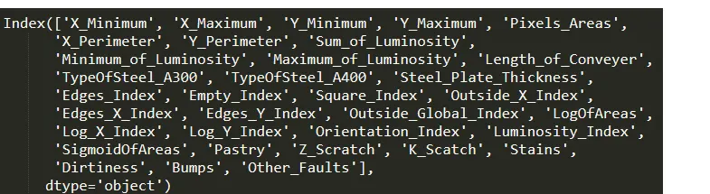
print('n',df.columns)
#To check for datatype and presence of null value for each column
print('n',df.info())
print('n',df.isnull().values.any())

#Last seven columns are type of error classification
label_columns = df.columns.values[-7:]
#Assigning the error classification values to variable targets
targets = (df.iloc[:,-7:]==1).idxmax(1)
print('n',label_columns)
print('n',targets)

#Dropping the 7 error classification columns and retaining only targets
dataset = df.drop(label_columns,axis=1)
#creating a new column 'target' with all classification values
dataset['target']=targets
print('n',dataset)
#Printing count of each type of error
print('n',dataset.target.value_counts())

fig, ax = plt.subplots(1,2,figsize=(15,6))
#Visualising the distribution of each error using histogram and pie chart
sns.countplot(x='target',data=dataset, ax=ax[0])
dataset['target'].value_counts().plot.pie(autopct = '%.1f', ax=ax[1])

#Visualising the correlation among each dataset feature
plt.figure(figsize=(10,11))
sns.heatmap(dataset.corr(),annot=False)

#Dropping features with high correlation to others
dataset=dataset.drop('TypeOfSteel_A400',axis=1)
dataset=dataset.drop('X_Minimum',axis=1)
dataset=dataset.drop('Y_Minimum',axis=1)

#Assigning feature column values to x
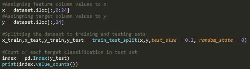
x = dataset.iloc[:,0:24]
#Assingning target column values to y 
y = dataset.iloc[:,24]

#Splitting the dataset to training and testing sets
x_train,x_test,y_train,y_test = train_test_split(x,y,test_size = 0.2, random_state = 0)

#KNN model
knn = KNeighborsClassifier(n_neighbors= 19)
knn.fit(x_train,y_train)
classfier = knn.fit(x_train,y_train)
print("nKNN accuracy:",knn.score(x_test,y_test))
plot_confusion_matrix(classfier,x_test,y_test,labels=None, sample_weight=None, normalize=None)
plt.show()

Code Explanation:

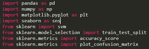
The modules needed to execute the program were imported.

Code Snippet:

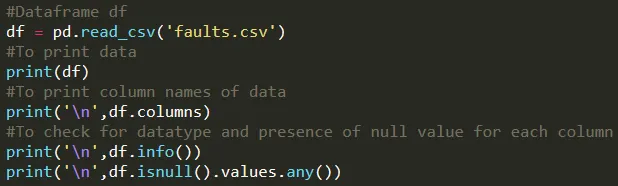
Exploratory data analysis was carried out on the given dataset.

Result:

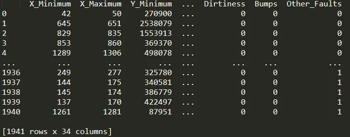
Printing the dataset:

Printing column names:

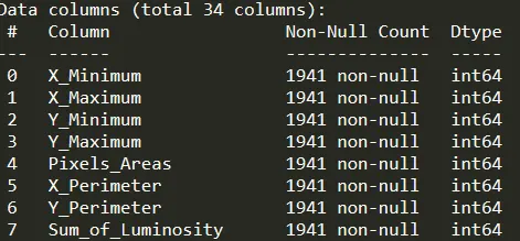
Printing data.info:

Checking for missing data:

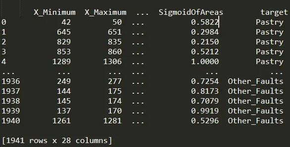
Conclusion: The dataset consists of 1941 instances and 34 columns. It does not have any missing data. The results are in one hot-encoded format.

Code Snippet:

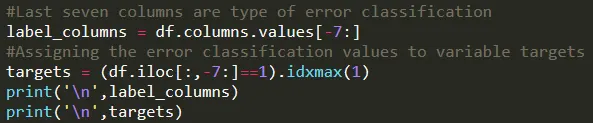
The last 7 columns were target classification. The column names were assigned to label_columns and all the values were indexed using df.iloc and assigned to variable targets.

Result:

Printing label_columns:

Printing targets:

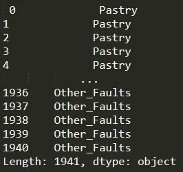
Code Snippet:

The 7 target columns were then dropped and a new column was created which consisted of all target values.

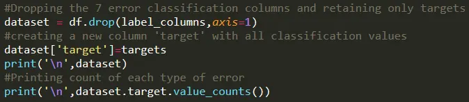
Result:

Printing new dataset:

Printing target counts:

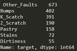
Code Snippet:

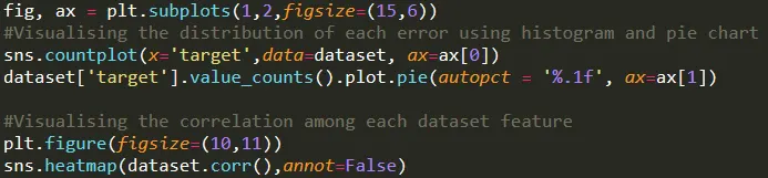
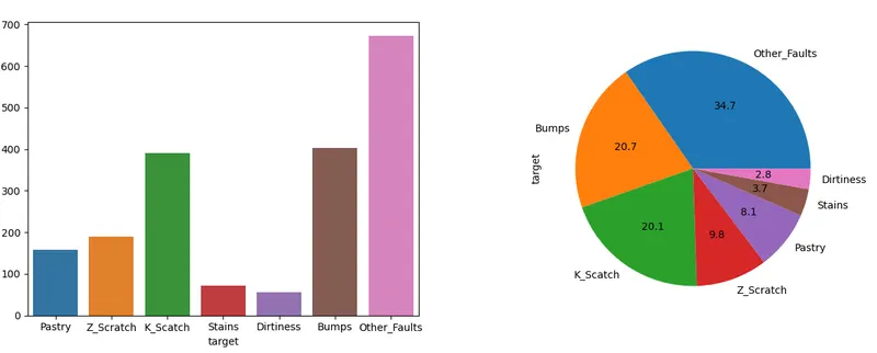
Visualizing the frequency of each target using countplot and plot.pie and the degree of correlation among the features using heatmap.

Result:

Visualising countplot and pieplot:

Heatmap:

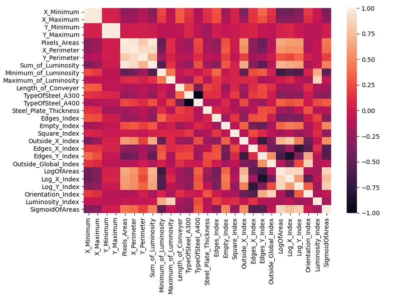
With the help of a heatmap, we can conclude that there is a high correlation between X minimum and X maximum, Y minimum and Y maximum, and type of steel A300 and A400.

Code Snippet:

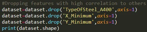
Based on our conclusions from the heatmap, we drop type of steel A400, X minimum and Y minimum.

Result

The shape of the dataset:

There are 1941 instances and 25 columns.

Code Snippet:

The feature values are assigned to variable x and target values to variable y.

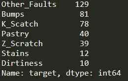
The x and y values are then split into training and testing sets. The test size is 20% of the size of the complete dataset.

The count of each target in the test set is printed using value_counts().

Result:

Code Snippet:

A variable knn is created and KNeighborsClassifier model is assigned to it. The knn model is trained with x train and y train values using knn.fit. Once the model is trained, the prediction accuracy of the model is observed.

Result:

The KNN model has an accuracy of 48.32%.

Confusion matrix: With the help of the confusion matrix, it is possible to understand which surface defects are being incorrectly classified.

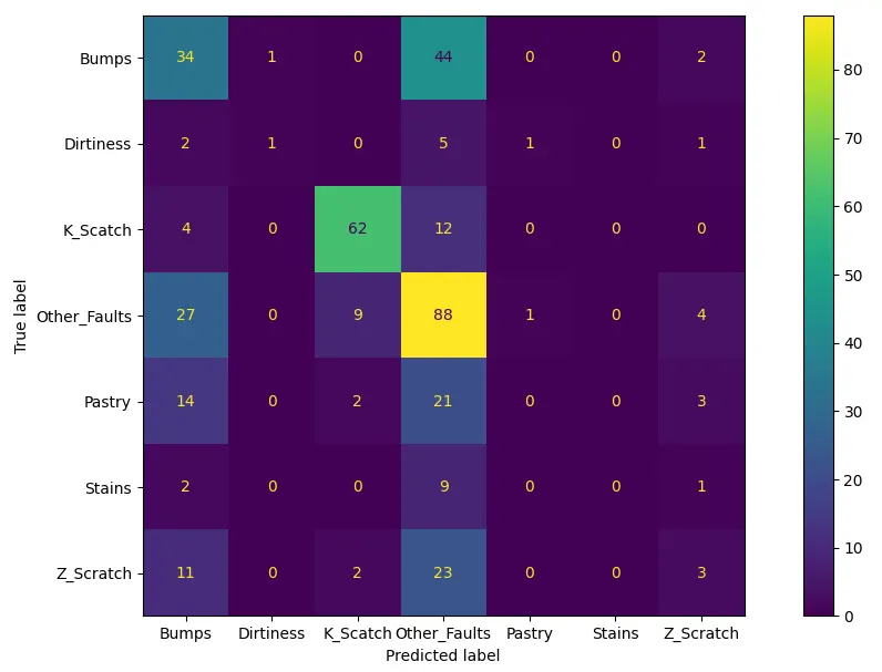
We can observe that majority of the faults are being falsely predicted as other faults. Therefore it is necessary to check the other faults values.

In comparison to the SVM model the accuracy obtained is less by a very small percentage.

Cofusion matrix comparison:

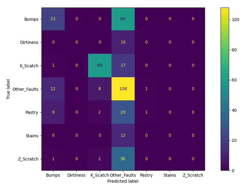
Conclusion: KNN model is able to predict bumps, K scratch and Z scratch more accurately but fails to predict 'other faults' correctly.