Supervised Learning - Classification Week 8 Challenge

Objectives:

• Pros and cons of K-Nearest Neighbours
• Application of K-NN algorithm to predict the surface defects in stainless steel plates.

a) Pros and cons of K-Nearest Neighbours

K-Nearest Neighbours (K-NN) is a supervised machine learning algorithm and it can be used for classification as well regression. It is non -parametric in nature as it doesn't make any assumption of the underlying data distribution pattern. It is also named as lazy algorithm as it doesn't have any training step as such. It predicts the cluster to which the new data point will based on feature similarity. In K-NN, "K" is a number and its a hyperparameter that can have significant impact on the result.

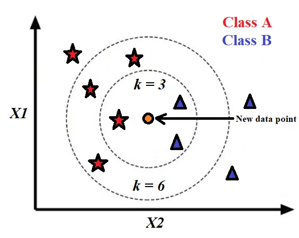
Figure 1. K-NN

Pros:

• Simple to understand and easy to implement.
• It is a non-parametric algorithm and hence, there is no assumptions.
• It can be used for classification as well as regression.
• There is flexibility for the user to select distance while building the model such as Euclidean Distance, Hamming Distance, Manhattan Distance, Minkowski Distance.

Cons:

• Computationally expensive as it searches for nearest neighbours for the new data point during prediction stage.
• Memory intensive as it stores all the data points.
• Highly sensitive to outliers and its accuracy is impacted by noise or irrelevant data.

b) Application of K-NN algorithm to predict the surface defects in stainless steel plates:

# Prediction of Surface defects on stainless steel plates through K-Nearest Neighbour Classifier

from sklearn import datasets, linear_model
from sklearn.metrics import confusion_matrix
import numpy as np
from sklearn.metrics import accuracy_score
from sklearn.model_selection import train_test_split

import pandas as pd

import seaborn as sns
import matplotlib.pyplot as plt
import warnings
warnings.filterwarnings("ignore")

from sklearn import preprocessing
from sklearn.preprocessing import StandardScaler

# Read the dataset
df = pd.read_csv('D:/MLnAI/Challenges/C5/faults.csv')
print(df.info())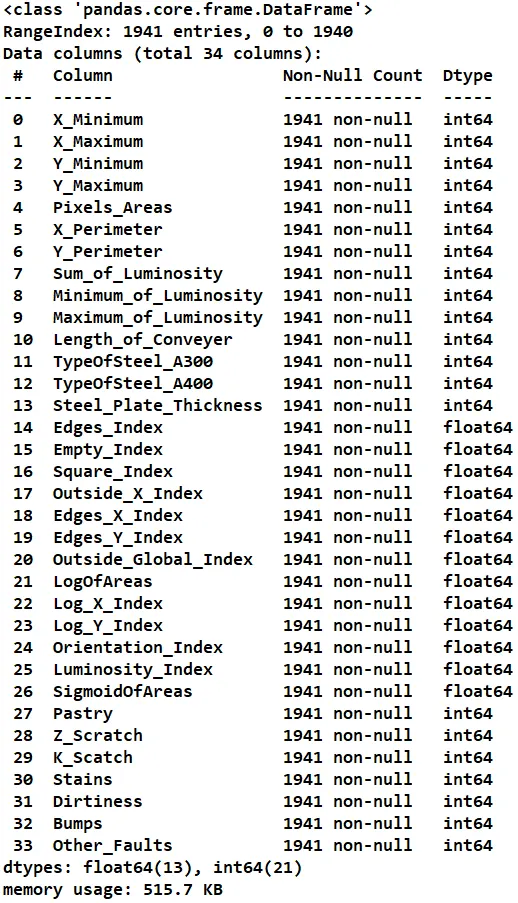

print(df.head(5))

print(df.describe(include="all"))

# Visualization through heatmap
sns.set(rc={'figure.figsize':(12,10)})
corr = df.corr()
sns.heatmap(corr, xticklabels=corr.columns.values,yticklabels=corr.columns.values)
plt.show()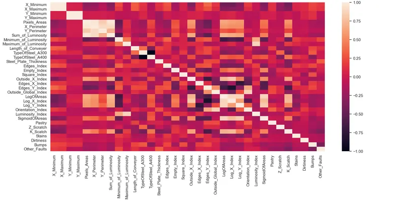

# Visualization through histograms
df.hist(figsize=(30,30))
plt.show()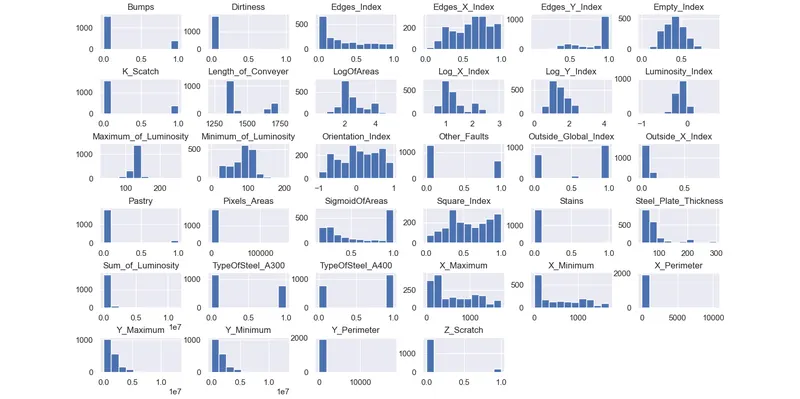

# Division of dataset into Features and faults
feat = df.values
fault_dataframe =df[["Pastry","Z_Scratch","K_Scatch","Stains","Dirtiness","Bumps","Other_Faults"]]
features = feat[:,0:27]
x = pd.DataFrame(features)

print(fault_dataframe.info())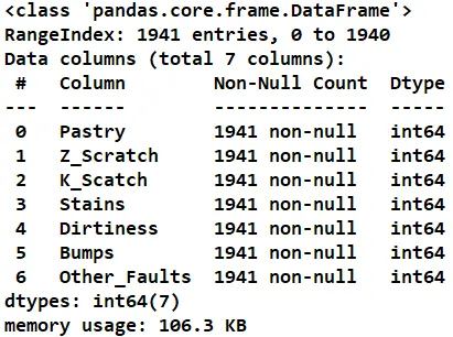

# Covert to single column with transpose
fault_single_col = []
for i in range(fault_dataframe.shape[0]):
    if fault_dataframe["Pastry"].values[i] == 1:
        fault_single_col.append("Pastry")
    elif fault_dataframe["Z_Scratch"].values[i] == 1:
        fault_single_col.append("Z_Scratch")
    elif fault_dataframe["K_Scatch"].values[i] == 1:
        fault_single_col.append("K_Scatch")
    elif fault_dataframe["Stains"].values[i] == 1:
        fault_single_col.append("Stains")
    elif fault_dataframe["Dirtiness"].values[i] == 1:
        fault_single_col.append("Dirtiness")
    elif fault_dataframe["Bumps"].values[i] == 1:
        fault_single_col.append("Bumps")
    else:
        fault_single_col.append("Other_Faults")

# Visualization through heatmap
sns.set(rc={'figure.figsize':(12,10)})
corr = fault_dataframe.corr()
sns.heatmap(corr, xticklabels=corr.columns.values,yticklabels=corr.columns.values)
plt.show()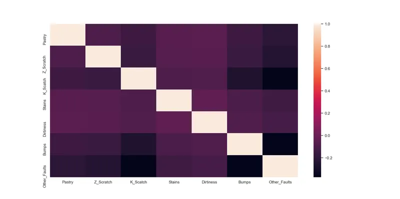

fault_single_col = np.array(fault_single_col)
print(fault_single_col.shape)

faultstype= pd.DataFrame({'faults':fault_single_col})
print(faultstype)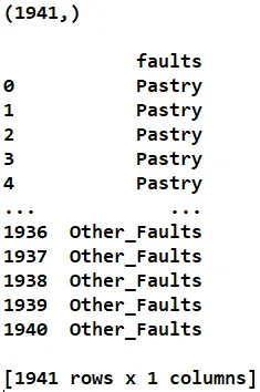

# Visualization through countplot
fig, ax=plt.subplots(1,2,figsize=(20,8))

faultstype['faults'].value_counts().plot.pie(ax=ax[0])
sns.countplot(x='faults', data=faultstype, ax=ax[1])
plt.show()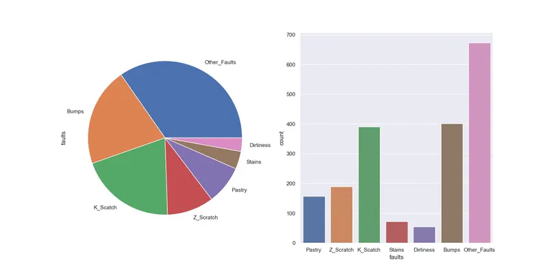

# Standardize the features in the datasets
sc=StandardScaler()
X=sc.fit_transform(x)
#print(X)

#Verify that the mean of each feature (column) is 0
#print("The mean is: ", X.mean(axis = 0))

#Verify that the mean of each feature (column) is 0
#print("The standard deviation is: ", X.std(axis = 0))

x_train, x_test, y_train, y_test = train_test_split(X, faultstype, test_size = 0.40, random_state = 1000)

#print ("x_train: ", x_train)
#print ("y_train: ", y_train)
#print("x_test: ", x_test)
#print ("y_test: ", y_test)

from sklearn.neighbors import KNeighborsClassifier
model = KNeighborsClassifier(n_neighbors=7)
print(model.fit(x_train, y_train))
print("The score is: ", model.score(x_test, y_test))
#print(model.predict(x_test))
#print(y_test)

The score is: 0.712998712998713

Y_predict = model.predict(x_test)
from sklearn import metrics
cm= metrics.confusion_matrix(y_test, Y_predict)
#print(cm)

# Visualization of confusion_matrix through heatmap
sns.set(rc={'figure.figsize':(12,10)})
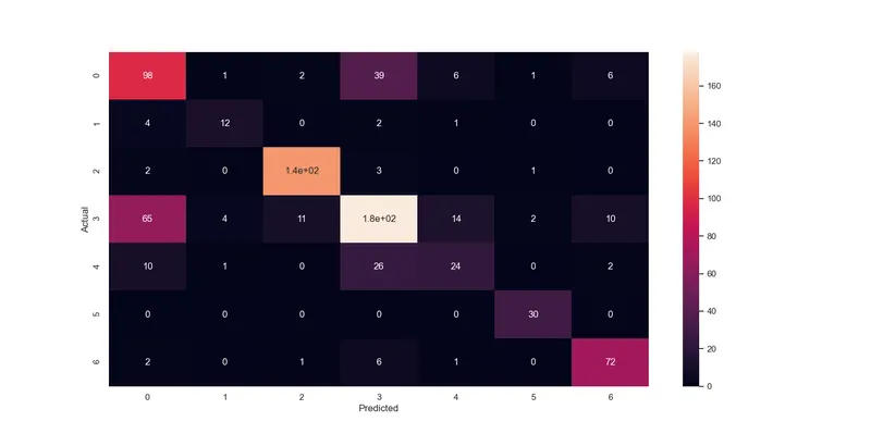
sns.heatmap(cm, annot=True)
plt.xlabel("Predicted")
plt.ylabel("Actual")
plt.show()