Supervised Learning - Classification Week 7 Challenge

NOTE: For this assignment Iris dataset is used.

First all the required libraries are imported and the dataset is loaded. Moreover, "target" column is added to the dataframe.

import numpy as np
import pandas as pd
import matplotlib.pyplot as plt
from sklearn.datasets import load_iris
from sklearn.metrics import confusion_matrix
from sklearn.metrics import classification_report
from sklearn.model_selection import train_test_split

iris = load_iris()

df = pd.DataFrame(iris.data,columns = iris.feature_names)
df["target"] = iris.target

Exploratory Data Analysis:

There are four features of the data. Let us look at "sepal length" behaviour on "target".

import seaborn as sns
sns.scatterplot(data = df, x = "sepal length (cm)",y="target")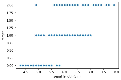

Here, the lengths of the sepal are over lapped for three variants of the target.

Lets add the categorical variant names as provided with the dataset.

df['species'] = pd.Categorical.from_codes(iris.target, iris.target_names)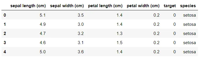

import seaborn as sns
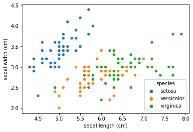
sns.scatterplot(data = df, x = "sepal length (cm)",y="sepal width (cm)", hue = 'species')

Let us look the scatter plot of sepal length and width.

Rather than looking at the individual plots seperately we can have the pair plot for all of the data.

sns.pairplot(data = df.drop(columns=['target']), hue = "species")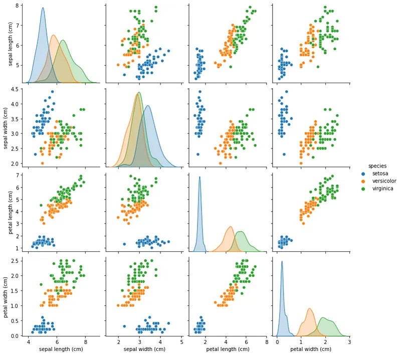

It is observed that the data are classified hence any of the classification algorithms can be used to predict the model.

There is one more way we can view the distribution of the data.

fig, axes = plt.subplots(1, 4, sharex=True, figsize=(15,5))
fig.suptitle('Distribution of Feature Data w.r.t Species')
sns.violinplot(data=df,x="species", y = "sepal length (cm)", ax=axes[0])
axes[0].set_title('Sepal length Vs Species')
sns.violinplot(data=df,x="species", y = "sepal width (cm)", ax=axes[1])
axes[1].set_title('Sepal width Vs Species')
sns.violinplot(data=df,x="species", y = "petal length (cm)", ax=axes[2])
axes[2].set_title('Petal length Vs Species')
sns.violinplot(data=df,x="species", y = "petal width (cm)", ax=axes[3])
axes[3].set_title('Petal width Vs Species')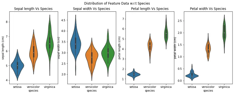

By looking at the plots above, we can say that the data of sepal length and width will be of least importance as it may lead to ambigous results because the data overlaps much in that feature.

Now lets select the data for training and test dataset.

X=df.drop(columns=['target','species'])
y = df['target']

# Splitting the dataset into the Training set and Test set
X_train, X_test, y_train, y_test = train_test_split(X, y, train_size = 0.6, random_state = 0)

Logistic Regression:

# LogisticRegression
from sklearn.linear_model import LogisticRegression
LogReg = LogisticRegression()
LogReg.fit(X_train, y_train)

y_pred_LogReg = LogReg.predict(X_test)

# Summary of the predictions made by the classifier
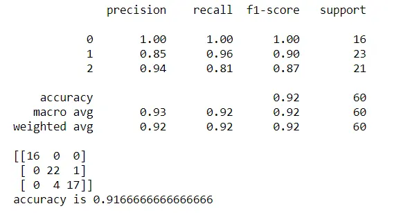
print(classification_report(y_test, y_pred_LogReg))
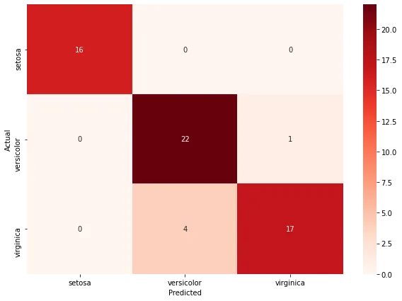
print(confusion_matrix(y_test, y_pred_LogReg))
# Accuracy score
from sklearn.metrics import accuracy_score
print('accuracy is',accuracy_score(y_pred_LogReg,y_test))

Output:

Support Vector Machine:

# Support Vector Machine's 
from sklearn.svm import SVC

SVM_C = SVC(kernel='linear')
SVM_C.fit(X_train, y_train)

y_pred_svm = SVM_C.predict(X_test)

# Summary of the predictions made by the classifier
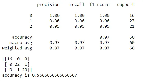
print(classification_report(y_test, y_pred_svm))
print(confusion_matrix(y_test, y_pred_svm))
# Accuracy score
from sklearn.metrics import accuracy_score
print('accuracy is',accuracy_score(y_pred_svm,y_test))

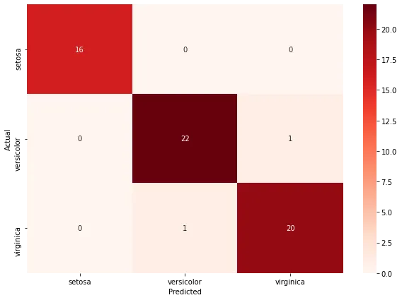
Output:

Decision Tree Classifier:

from sklearn.tree import DecisionTreeClassifier

DTC = DecisionTreeClassifier()

DTC.fit(X_train, y_train)

y_pred_DTC = DTC.predict(X_test)

# Summary of the predictions made by the classifier
print(classification_report(y_test, y_pred_DTC))
print(confusion_matrix(y_test, y_pred_DTC))
# Accuracy score
from sklearn.metrics import accuracy_score
print('accuracy is',accuracy_score(y_pred_DTC,y_test))

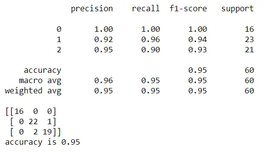
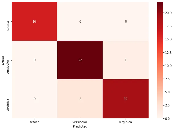
Output:

Feature Important Score:

# view the feature scores

feature_scores = pd.Series(DTC.feature_importances_, index=X_train.columns).sort_values(ascending=False)

feature_scores
# Creating a seaborn bar plot

sns.barplot(x=feature_scores, y=feature_scores.index)



# Add labels to the graph

plt.xlabel('Feature Importance Score')

plt.ylabel('Features')



# Add title to the graph

plt.title("Visualizing Important Features")



# Visualize the graph

plt.show()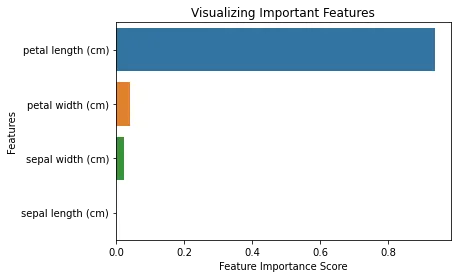

As observed from our analysis previously, sepal length and width are least significant features, even from the modeling of decision tree classifier.

ROC Curve and AUC values:

from sklearn.metrics import roc_curve
#from sklearn.metrics import roc_auc_curve

y_true = y_test
y_probas1 = y_pred_DTC# predicted results
y_probas2 = y_pred_svm# predicted results
y_probas3 = y_pred_LogReg# predicted results

fpr1, tpr1, thresholds1 = roc_curve(y_true, y_probas1 , pos_label=2)
fpr2, tpr2, thresholds2 = roc_curve(y_true, y_probas2, pos_label=2)
fpr3, tpr3, thresholds3 = roc_curve(y_true, y_probas3, pos_label=2)
# Print ROC curve
plt.plot(fpr1,tpr1,'c', label='DecisionTree')
plt.plot(fpr2,tpr2,'b', label='SupportVectorMachine')
plt.plot(fpr3,tpr3,'r', label='LogisticRegression')
plt.plot([0,1],[0,1],'k--')
plt.xlabel('False Positive Rate')
plt.ylabel('True Positive Rate')
plt.legend()
plt.show() 

# Print AUC
auc3 = np.trapz(tpr3,fpr3)
auc2 = np.trapz(tpr2,fpr2)
auc1 = np.trapz(tpr1,fpr1)

print('The AUC: {0} % using Decision Tree Classifier'.format(auc1*100))
print('The AUC: {0} % using SVM'.format(auc2*100))
print('The AUC: {0} % using Logistic Regression'.format(auc3*100))

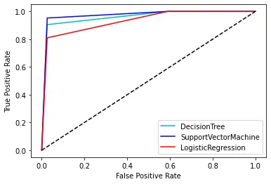
It can be observed from the above plot that AUC under Support vector machine ROC is higher and the same was deduced from higher accuracy of the model. Thus, the developed SVM model is better of the other classifiers for this data.

acc=[accuracy_score(y_pred_DTC,y_test),accuracy_score(y_pred_svm,y_test),accuracy_score(y_pred_LogReg,y_test)]
models = ['Decision Tree','Support Vector Machine','Logistic Regression']
acc_ = np.array(acc)*100
sns.barplot(acc_, models,)
plt.xlim([90,100])
plt.xlabel('Accuracy %')
plt.title('Classifier Accuracy')
plt.show()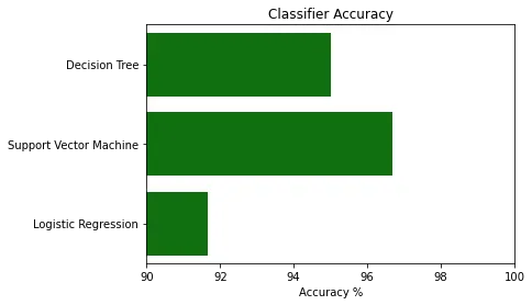

It can be observed from the above plot that AUC under Support vector machine ROC is higher and the same was deduced from higher accuracy of the model. Thus, the developed SVM model is better of the other classifiers for this data.

Pros:

• It works really well with a clear margin of separation
• It is effective in high dimensional spaces.
• It is effective in cases where the number of dimensions is greater than the number of samples.
• It uses a subset of training points in the decision function (called support vectors), so it is also memory efficient.

Cons:

• It doesn’t perform well when we have large data set because the required training time is higher
• It also doesn’t perform very well, when the data set has more noise i.e. target classes are overlapping
• SVM doesn’t directly provide probability estimates, these are calculated using an expensive five-fold cross-validation. It is included in the related SVC method of Python scikit-learn library.