Challenge

Supervised Learning - Classification Week 7 Challenge

Q1.

Pros of SVM:

Effective in high-dimensional spaces: SVM is particularly powerful in handling data with many features, especially in scenarios where the number of dimensions exceeds the number of samples.
Works well for small datasets: SVM is effective when the dataset is relatively small but well-labeled, making it suitable for scenarios where data collection is difficult or expensive.
Clear decision boundaries: SVM creates a maximum margin hyperplane, which ensures that the model is robust and generalizes well to new data, thus reducing the risk of overfitting.
Versatile kernel trick: By using different kernel functions (e.g., linear, polynomial, radial basis function), SVM can model complex, non-linear decision boundaries, making it a flexible model for a variety of tasks.
Works well with binary classification: SVM is ideal for binary classification problems and can efficiently handle linearly separable as well as non-linearly separable data through the use of kernel methods.

Cons of SVM:

Slow for large datasets: SVM’s complexity is highly dependent on the size of the dataset. Training times can become prohibitively slow when dealing with large-scale datasets.
Sensitive to the choice of kernel: Selecting the right kernel and its corresponding parameters (such as the penalty parameter C and the kernel coefficient γ for the RBF kernel) requires careful tuning and can significantly affect model performance.
Memory-intensive: SVM can require a lot of memory, especially for large datasets, as it retains a subset of the training points (called support vectors) in memory for making predictions.
Does not directly provide probability estimates: Unlike some other classifiers, SVM does not naturally output probabilities for predictions. Probabilities can be estimated using techniques like Platt scaling, but this adds complexity.
Not well-suited for noisy data or overlapping classes: If there is significant overlap between classes or noisy data, SVM may struggle to find a clear margin and could misclassify points, especially without proper tuning of the soft margin parameter C

Q2.

To apply SVM algorithm on the surface defects in stainless steel plates dataset and evaluate it

Descriptive analysis :

The given data is imported in jupyter notebook

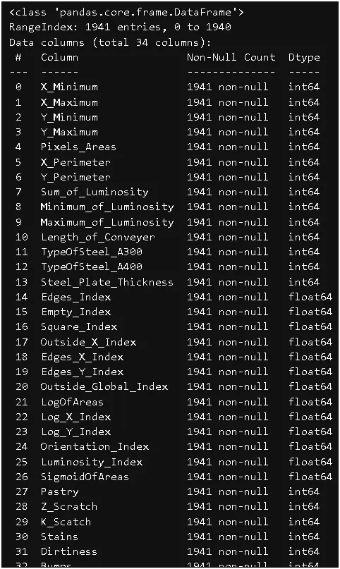
So there are 1941 rows and 34 columns.

We check for null values and found there are no null values

Since there are many features we can remove some features which almost similar to other features, we can find this by plotting a correlation matrix

So the areas which are close to the value 1 are closely related and hence can be removed to avoid repetition in the features

From the above figure we can say that

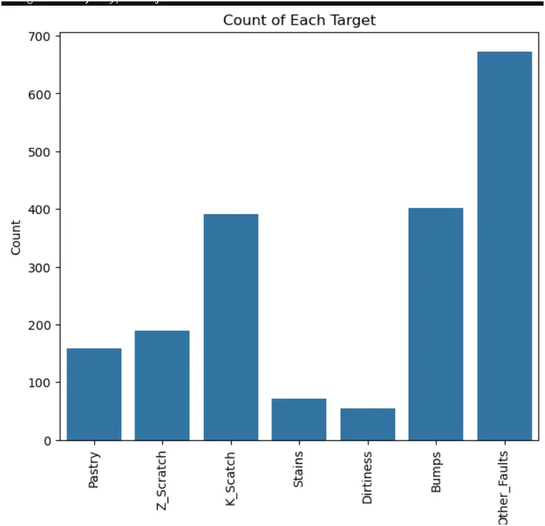
We can see the counts of each fault with other_faults having the maximum count

Code is in Ipynb File

Ship work like this
in your own course.