Supervised Learning - Classification Week 7 Challenge

1)

Objective:

• Brief explaination on Support Vector Machine (SVM). Pros and cons.
• SVM application to “Surface defects in stainless steel plates” dataset and its evaluation.

a) Support Vector Machine (SVM)

The SVM algorithm was invented by Vladimir N. Vapnik and Alexey Ya. Chervonenkis in 1963. SVMs comes under the supervised machine learning models and it can be applied to classification (SVC — Support Vector Classification) as regression (SVR — Support Vector Regression) problems. SVMs are commly used for classification problems and hence more emphasis will be given for SVC here. Few important key terms related to SVMs are explained below:

Hyperplane:

The SVCs aim to find the best hyperplane (also called decision boundary) that best separates (splits) a dataset into two classes/groups (binary classification problem). Depending of the number of the input features/variables, the decision boundary can be a line (if we had only 2 features) or a hyperplane if we have more than 2 features in our dataset.

Support Vectors (SV):

SV are the samples (data-points) that are located nearest to the separating hyperplane. The location of hyperplane is altered on the basis of these samples, in the event of their removal. Hence, these samples are very important to define the location and orientation of best decision boundary.

Support Vector Machine Margin:

SVM margin is the distance between the hyperplane and the nearest data points. The aim is to choose a hyperplane with the greatest possible margin. SVM algorithm selects the decision boundary which maximises the margin. If the decision boundary is too close to the support vectors, the model would not generalise well. To better generalise the model, the idea of soft margin is implemented. It allows some samples to be misclassified or be on the wrong side of decision boundary.

The soft margin tries to solve the folowing optimization problem:

1. Maximise the margin
2. Maximise the number of samples correctly classified.

This trade-off between two optimization goals are controlled by a term called C-parameter.

As long as we deal with a linearly separable dataset, the job of SVM is relatively easy. Although, real life examples often provided us with linearly non-seperable datasets. The kernel trick is utlized in such conditions. The kernel trick maps the original data points in a higher dimensional space in order to make them linearly separable in that space.

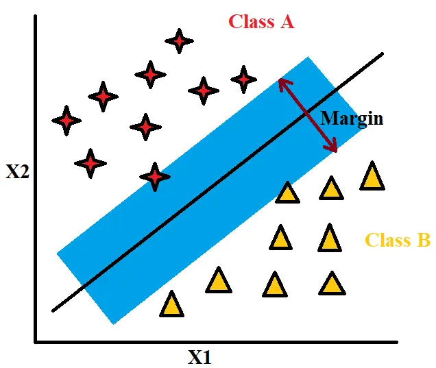
Figure 1. Support Vector Machine (SVM) methodology

Pros:

• It works really well with clear margin of separation and high dimesional space.
• It offers good accuracy and faster prediction.
• Effective in cases where number of dimensions is greater than the number of samples
• It is memory efficient as it uses a subset of training points in the decision function (called support vectors).

Cons:

• It doesn’t perform well when we have large data set because the required training time is higher.
• It also doesn’t perform very well, when the data set has more noise i.e. target classes are overlapping.
• SVM doesn’t directly provide probability estimates, these are calculated using an expensive five-fold cross-validation.

2)

 Prediction of Surface defects on stainless steel plates through Support Vector Classifier

from sklearn import datasets, linear_model
from sklearn.metrics import confusion_matrix
import numpy as np
from sklearn.metrics import accuracy_score
from sklearn.model_selection import train_test_split

import pandas as pd

import seaborn as sns
import matplotlib.pyplot as plt
import warnings
warnings.filterwarnings("ignore")

from sklearn import preprocessing
from sklearn.preprocessing import StandardScaler

# Read the dataset
df = pd.read_csv('D:/MLnAI/Challenges/C4/faults.csv')
print(df.info())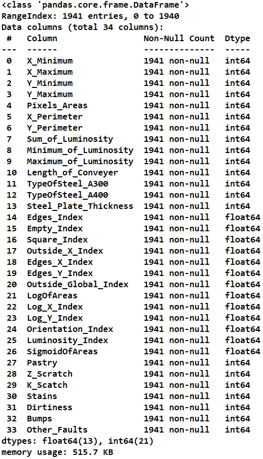

print(df.head(5))

Displaying the first five rows of the dataset

print(df.describe(include="all"))

# Visualization through heatmap
sns.set(rc={'figure.figsize':(12,10)})
corr = df.corr()
sns.heatmap(corr, xticklabels=corr.columns.values,yticklabels=corr.columns.values)
plt.show()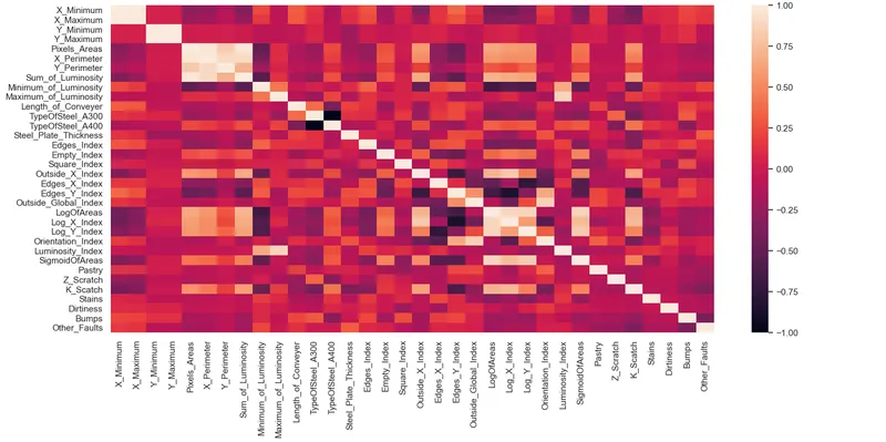

# Visualization through histograms
df.hist(figsize=(30,30))
plt.show()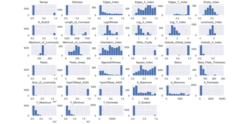

# Division of dataset into Features and faults
feat = df.values
fault_dataframe =df[["Pastry","Z_Scratch","K_Scatch","Stains","Dirtiness","Bumps","Other_Faults"]]
features = feat[:,0:27]
x = pd.DataFrame(features)

print(fault_dataframe.info())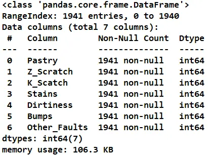

# Covert to single column with transpose
fault_single_col = []
for i in range(fault_dataframe.shape[0]):
    if fault_dataframe["Pastry"].values[i] == 1:
        fault_single_col.append("Pastry")
    elif fault_dataframe["Z_Scratch"].values[i] == 1:
        fault_single_col.append("Z_Scratch")
    elif fault_dataframe["K_Scatch"].values[i] == 1:
        fault_single_col.append("K_Scatch")
    elif fault_dataframe["Stains"].values[i] == 1:
        fault_single_col.append("Stains")
    elif fault_dataframe["Dirtiness"].values[i] == 1:
        fault_single_col.append("Dirtiness")
    elif fault_dataframe["Bumps"].values[i] == 1:
        fault_single_col.append("Bumps")
    else:
        fault_single_col.append("Other_Faults")

# Visualization through heatmap
sns.set(rc={'figure.figsize':(12,10)})
corr = fault_dataframe.corr()
sns.heatmap(corr, xticklabels=corr.columns.values,yticklabels=corr.columns.values)
plt.show()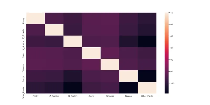

fault_single_col = np.array(fault_single_col)
print(fault_single_col.shape)

faultstype= pd.DataFrame({'faults':fault_single_col})
print(faultstype)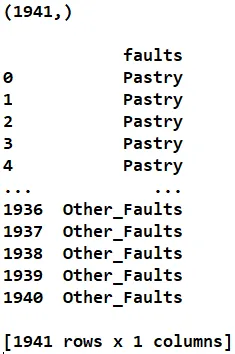

# Visualization through countplot
fig, ax=plt.subplots(1,2,figsize=(20,8))

faultstype['faults'].value_counts().plot.pie(ax=ax[0])
sns.countplot(x='faults', data=faultstype, ax=ax[1])
plt.show()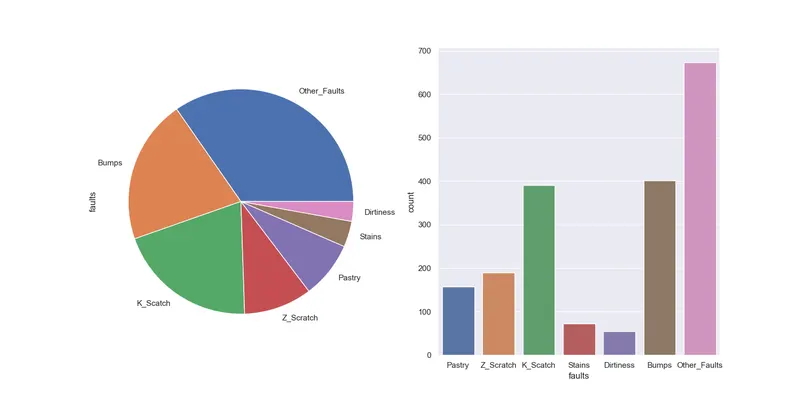

# Standardize the features in the datasets
sc=StandardScaler()
X=sc.fit_transform(x)
#print(X)

#Verify that the mean of each feature (column) is 0
#print("The mean is: ", X.mean(axis = 0))

#Verify that the mean of each feature (column) is 0
#print("The standard deviation is: ", X.std(axis = 0))

x_train, x_test, y_train, y_test = train_test_split(X, faultstype, test_size = 0.40, random_state = 1000)

#print ("x_train: ", x_train)
#print ("y_train: ", y_train)
#print("x_test: ", x_test)
#print ("y_test: ", y_test)

from sklearn.svm import SVC
model = SVC(gamma='auto')
print(model.fit(x_train, y_train))
print("The score is: ", model.score(x_test, y_test))
#print(model.predict(x_test))
#print(y_test)

Y_predict = model.predict(x_test)
from sklearn import metrics
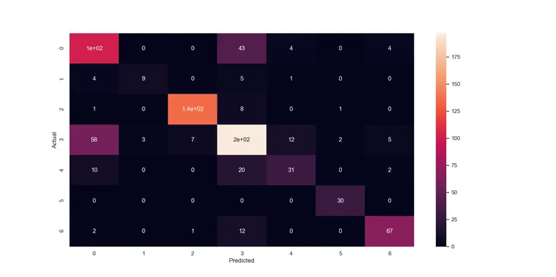
cm= metrics.confusion_matrix(y_test, Y_predict)
#print(cm)

The score is: 0.7361647361647362

# Visualization of confusion_matrix through heatmap
sns.set(rc={'figure.figsize':(12,10)})
sns.heatmap(cm, annot=True)
plt.xlabel("Predicted")
plt.ylabel("Actual")
plt.show()