Steady Vs Unsteady flow over a cylinder

Aim – Two dimensional CFD analysis of flow over a cylinder using Ansys 2020 R2.

Introduction –

Flow over a cylinder is one of the most extensively fluid dynamics problems studied, both experimentally and numerically. Intensive investigations are still performed due to the complex dynamics of the wake flow. Cross flow normal to the axis of the cylinder is encountered in a variety of engineering applications. The shape of the cylinder is quite simple but the underlying physics of the flow is quite complex.

A computational study has been performed to understand the effect of Reynolds number on the flow physics.

Thus, due to its wide applications a computational study has been performed in the present work using Ansys Fluent Student Version (Version 2020 R2).

Modelling and Solving approach –

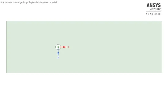
Solid Model – A 2D surface was developed in Ansys Spaceclaim. The pull feature of Spaceclaim was utilized to separate the cylinder geometry from the domain geometry. The cylinder diameter is 2 m. The length and height of the domain is 30D and 10D respectively. The surface created in Spaceclaim is shown below.

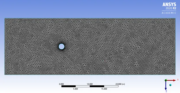
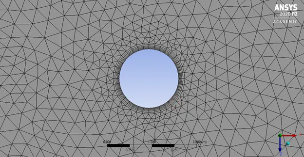
2. Meshing – Ansys Meshing was used to create the mesh using tetrahedral elements for a simple study. The below table highlights the mesh details. The meshed geometry is also shown below.

Element size	0.5 m
Number of divisions on the cylinder	36
Inflation layers	6

Solver Settings – Ansys Fluent was used as the solver. Both steady state and transient computational studies have been performed using a pressure based solver. A custom fluid was used. The density was taken as 1 kg/m3 and viscosity as 0.05 kg/m-s.

Boundary conditions – Reynolds number was varied by changing the inlet velocities. The below table highlights the different velocities used.

Reynolds Number	Type of study	Inlet velocity (m/s)	Gage Pressure at outlet	Top and bottom wall of the domain
10	Steady	0.25	0	Symmetry
100	Steady and transient	2.5	0	Symmetry
1000	Steady	25	0	Symmetry
10000	Steady	250	0	Symmetry
100000	Steady	2500	0	Symmetry

Computational model – Since the Reynolds number lie below in the laminar regime for flow over a cylinder, laminar viscous model has been used in all the cases.

Spatial Discretization Method – SIMPLE Pressure velocity coupling scheme was used to solve the Navier Stokes Equations. The methods used for spatial discretization of each of the terms for both steady and unsteady simulation is given in the below table –

Term/Equation	Method
Gradient	Least Squares Cell based
Pressure	Second Order
Momentum	Second Order Upwind

Results and Discussion – The wake flow physics for flow over a cylinder is a function of Reynolds number.

When Reynolds number is below 40, the entire flow domain is symmetric about the cylinder center. However, as the Reynolds number is increased beyond this, unstable and transverse oscillation of vortices start. This phenomenon is known as vortex shedding. The series of vortices beside the cylinder for the Von Karman Vortex Street. It is important to perform the analysis of vortices because if in practical situations, the oscillation frequency matches with the resonance frequency of an object, it can lead to catastrophic situations (Tacoma Narrows Bridge).

Steady state simulations –

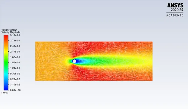
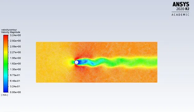
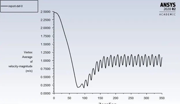
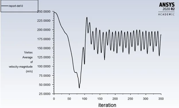
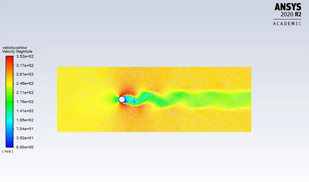
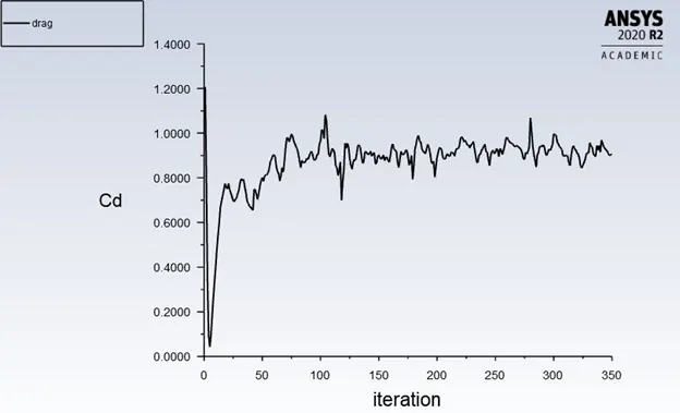
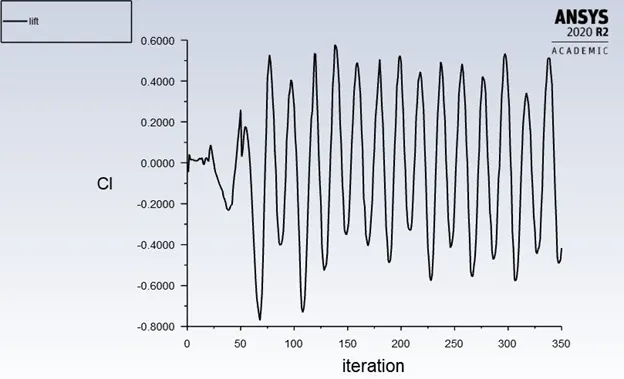
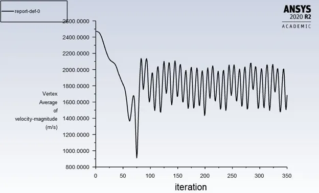
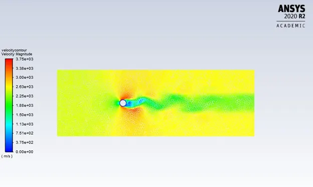
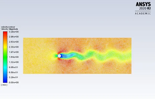
It can be observed from the fluctuations in velocity contours and vertex point average of velocity that von Karman vortices tend to develop at Reynolds number of 100 and above. At Re = 10, the flow is symmetric about the cylinder center.

From the velocity contours of the steady state simulations, it is clear that formation of vortices start at Re = 100 (Re = 40 is critical, but not considered here). Also, as the Reynolds number is increased the separation of BL is delayed due to the onset of turbulence in the vortices.

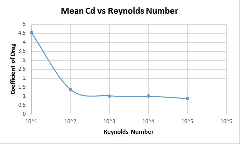
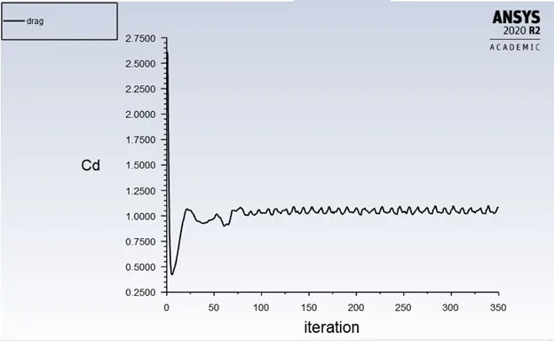
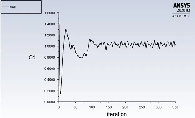
The variation of drag coefficient with Reynolds number has also been shown here.

Reynolds Number	Mean coefficient of Drag
10	4.548
100	1.381
1000	1.024
10000	1.000
100000	0.874

Validation study – To assess the accuracy of the computational study, the mean drag force at Re = 100 was compared to that available in literature. The findings is given in the below table.

Source of result	Mean Cd at Re = 100
Present 2D computation	1.381
2D computation (Rajani et al [1])	1.335
Error%	3.44

An error of just 3.44% in our numerical computation clearly indicates the high accuracy of the model.

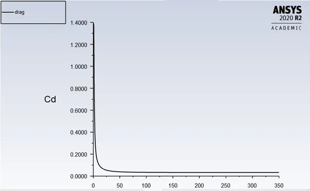
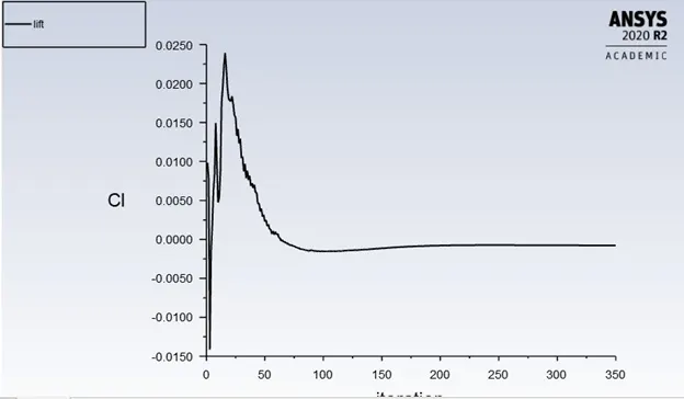
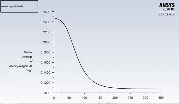
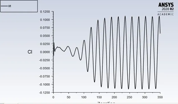
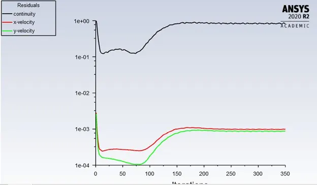
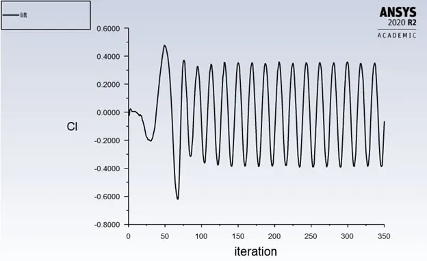
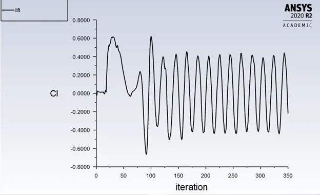
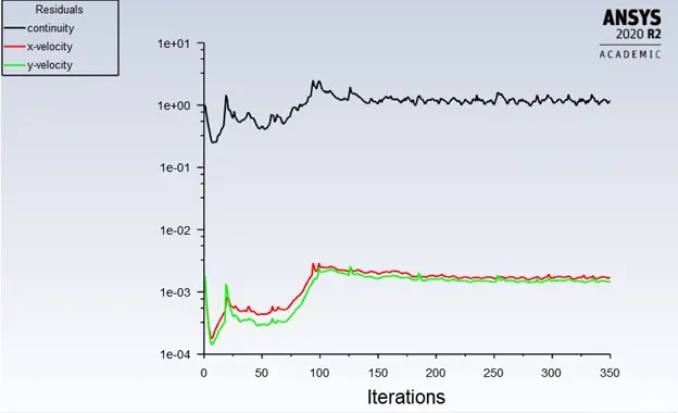
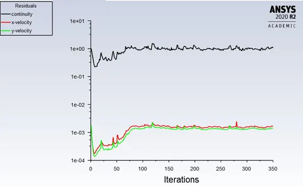
Some important variables for engineering computations are coefficient of drag, lift and Strouhal number (only for transient case). These plots have also been shown below.

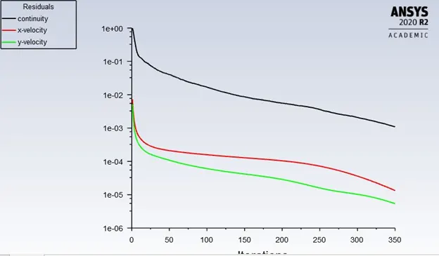
The solution has been considered to be converged once the velocity fluctuations become periodic.

The plots for different Reynolds number are –

Re = 10

Re = 100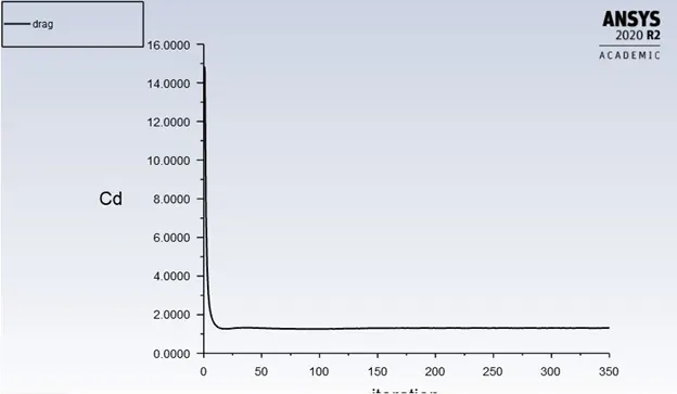

Re = 1000

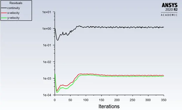
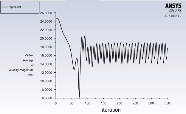
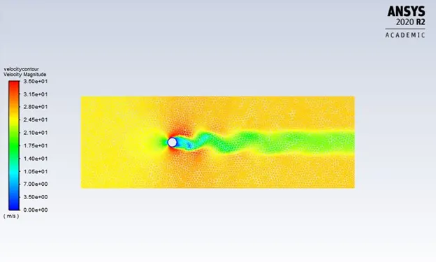
Re = 10000

Re = 100000

Transient simulations –

The following are the solver settings for transient simulation at Re = 100.

Time step size	0.1
Number of time steps	950
Transient formulation	First order implicit

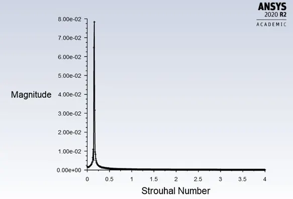
Vortex shedding is inherently a transient phenomenon. Thus, to get an accurate picture of the flow, a transient study was also performed at Re = 100. The mean Cd and Strouhal Number (from Fast Fourier Transform technique in Fluent) have been compared with that given by Rajani et al. [1].

	Mean Coefficient of Drag	Strouhal Number
Present study	1.381	0.159
Rajani et al. [1]	1.335	0.157
Error %	3.445	1.275

Strouhal Number - The flow process in the wake of a cylinder or tube involves the formation and shedding of vortices alternately from one side and then the other. This phenomenon is of major importance in engineering design because the alternate formation and shedding of vortices also creates alternating forces, which occur more frequently as the velocity of the flow increases.

When the frequency is in the audible range, a sound can be heard and the body appears to sing. Resonance may occur if the vortex shedding frequency is near the structural-vibration frequency of the body. A dimensionless number, the Strouhal number Sr, is commonly used as a measure of the predominant shedding frequency fs. The definition is

Where L is a characteristic length (equal to the diameter D in case of a circular cylinder or tube in cross flow) and U is the freestream velocity.

FFT for calculating Strouhal Number –

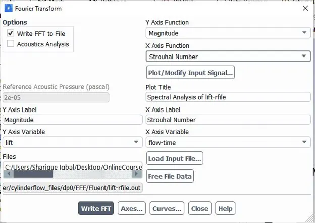
1. Select the FFT tab in results section of fluent.
2. In the window that appears, chose the following options and click plot (instead of Write FFT option shown here). The lift coefficient file available in the folder where all the simulation files have been stored should be loaded.

The Strouhal number plot can then also be written using the write FFT option.

Plots at Re = 100

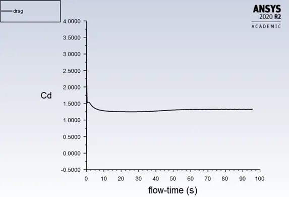
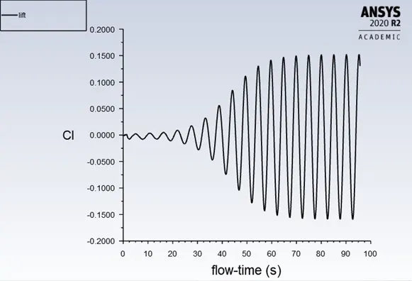
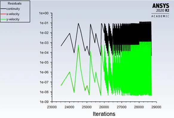
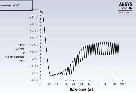
The vertex average of velocity starts periodic behaviour after a flow time of about 65 sec which is an indication that steady state has been reached.

From the Strouhal number plot, the St = 0.159 corresponding to the peak Y-axis value.

References –

1. Rajani et al, Numerical Simulation of Laminar Flow Past a circular cylinder. 2008.