Steady Vs Unsteady flow over a cylinder

Question :

Simulate the flow over a cylinder and explain the phenomenon of Karman vortex street.

PART-I

1. Simulate the flow with the steady and unsteady case and calculate the Strouhal Number for Re= 100.

PART-II

1. Calculate the coefficient of drag and lift over a cylinder by setting the Reynolds number to 10,100,1000,10000 & 100000. (Run with steady solver)
2. Discuss the effect of Reynolds number on the coefficient of drag. [ Results should be validated with any standard literature and error should be within 5 %]

Expected results:-

1. In both approaches, show that the flow has converged. That is, what quantities or plots need to be looked at to determine that the flow has converged?
2. Plots of the coefficient of drag and lift.
3. Plots to show vortex shedding behind the cylinder.
4. Mention the preferred material at the end of the challenge submission page.

Given:

PART-I

Re= 100.

PART-II

Reynolds number = 10,100,1000,10000 & 100000. (Run with steady solver)

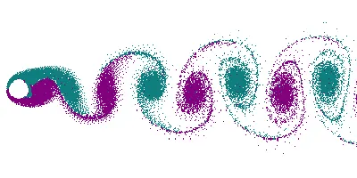
Karman vortex street :

It is a phenomena in which if a flow is disturbed by a body it generates repeating pattern of swirling vortices. Major 2 parametersresponsible for this are velocity and reynolds number. This will happen after certain reynolds number i.e. 90+ at some range of velocities.

Simulation Procedure :

1] First we need to start the workbench and select fluid flow (fluent) solver. Then setup the steps shown in fluent solver as follows.

Geometry

1. Open Geometry section which will be done through spaceclaim.
2. Now create the geometry according to given dimensions.
3. Then select the cylinder and delete it, Also delete the extra lines.
4. This completes the Geometry section.

Mesh

1. Open the Mesh from Workbench.
2. Now change the element size and generate mesh (Here we have used 0.3m as element size).
3. By default, Quadrilateral mesh is created, so we need to go in mesh/method, select mesh body and change the mesh into Triangular mesh.
4. Again go in mesh and select sizing and add the no. of divisions to edge of cylinder so the cylinder becomes more smooth (we have added 36 divisions in our case).
5. Then again same way we have to go in mesh and select inflation to add inflation layer for a quality mesh. Here we are using first layer thickness and layer size as 5e-3 with 1.2 growth rate for 6 layers. For this we have to select the body first and then the edge of cylinder to create the layers at the cylinder edge.
6. Lastly, we need to name the Boundaries like Inlet, Outlet, Symmetry and Wall. This completes the Mesh section.

Setup

1. Open the Setup from Workbench.
2. First perform the mesh check which is present in domain section.
3. Now get in physics section and check the viscous model if its laminar which by default will be laminar, if not then set it to laminar.
4. Then create user material and change its density and viscosity according to the given specifications. Delete the default air material.
5. Set the boundaries like inlet velocity to 1m/s, outlet pressure etc.
6. Now go to result section and create a point at x= 8m from center of cylinder to the right side of cylinder. Nmae the point.
7. Go back to solution section and create report definitions.
8. first create vertex average of velocity magnitude at monitor point. Then create drag and lift coefficient definitions.
9. Set the solution method to SIMPLE and then set the solver as STEADY/LAMINAR according to requirement.
10. After that initialize it, for steady we use HYBRID initializing and for transient we use STANDARD initailizing.
11. Go to result section and add 2 new contours i.e velocity and pressure.
12. Now create solution animation for velocity.
13. Lastly, run the simulation for some iterations and note down the values of lift, drag, etc. This completes Setup part.

Result

1. Select the wall volume to make it visible.
2. After that, insert the plane and color it with variable like pressure and velocity which shows the pressure and velocity flow on plane.
3. Edit the legend according to requirement. this completes the results and hence the entire simulation.

2] we are goint o run 2 cases

• first one with steady and trasient solver at Reynolds number = 100
• Second with steady solver at reynolds number = 10/100/1000/10000/100000.

DOMAIN:

MESH :

We are using element size as 0.3m.

Inflation layers

PART I

In part I we will run steady and transient solver for reynolds number 100.

RESULTS of STEADY STATE

• Residual

• Vertex Average

• Coefficient of drag

• Coefficient of Lift

• Velocity Contour

• Pressure Contour

RESULTS OF TRANSIENT STATE

• Residual

• Vertex Average

• Coefficient of Drag

• Coefficient of Lift

• Velocity Contour

• Pressure Contour

• Drag and Lift Coefficient Table:

	STEADY SOLVER	TRANSIENT SOLVER
Coefficient of Drag	1.37	1.37
Coefficient of Lift	0.16	-0.206

Strouhal Number : The Strouhal number represents the ratio of inertial forces due to the local acceleration of the flow to the inertial forces due to the convective acceleration. Depending on the time scale of the problem, this ratio may be of order unity, and therefore its importance is not obvious.

for steady state we cannot calculate strouhal number because there is no time parameter.

for transient state strouhal number plot is shown below,

strouhal number = 0.15

• Strouhal Number plot (Transient case)

PART II

In part II we will run steady solver for reynolds number 10/100/1000/10000/100000. We will run them for 1000 iterations.

• RESULTS

1] Reynolds Number = 10

• Residual

• Vertex Average

• Coefficient of Drag

• Coefficient of Lift

• Velocity Contour

• Pressure Contour

2] Reynolds Number = 100

• Residual

• Vertex Average

• Coefficient of Drag

• Coefficient of Lift

• Velocity Contour

• Pressure Contour

3] Reynolds Number = 1000

• Residual

• Vertex Average

• Coefficient of Drag

• Coefficient of Lift

• Velocity Contour

• Pressure Contour

4] Reynolds Number = 10000

• Residual

• Vertex Average

• Coefficient of Drag

• Coefficient of Lift

• Velocity Contour

• Pressure Contour

5] Reynolds Number = 100000

• Residual

• Vertex Average

• Coefficient of Drag

• Coefficient of Lift

• Velocity Contour

• Pressure Contour

Tabular result for drag and lift coefficient of various reynolds number is given below

Reynolds Number	Coefficient of Drag	Coefficient of Lift
10	3.32	-0.0014
100	1.37	0.1610
1000	0.7547	-0.5594
10000	0.7319	-0.2779
100000	0.7782	-0.6963

CONCLUSION :

• From above results we can see that as the reynolds number increases the drag coefficient decreases.
• We can also see in residual plots that after some no. of iterations flow gets converged which can be seen when the residual pattern gets constant like in reynolds number = 1000 residual pattern where it gets constant after 275 iterations, or when the spcified convergence range is crossed by all residual values then the flow will get converged like in residual plot of reynolds number = 10 plot where after 598 iterations the flow gets converged because all residual values go below convergence value i.e 1e-03.
• Transient simulation can ce considered over steady as it is time dependent and more accurate for this problem.