Speed Programming in Matlab/Octave for non computer science engineers(simple pendulum)

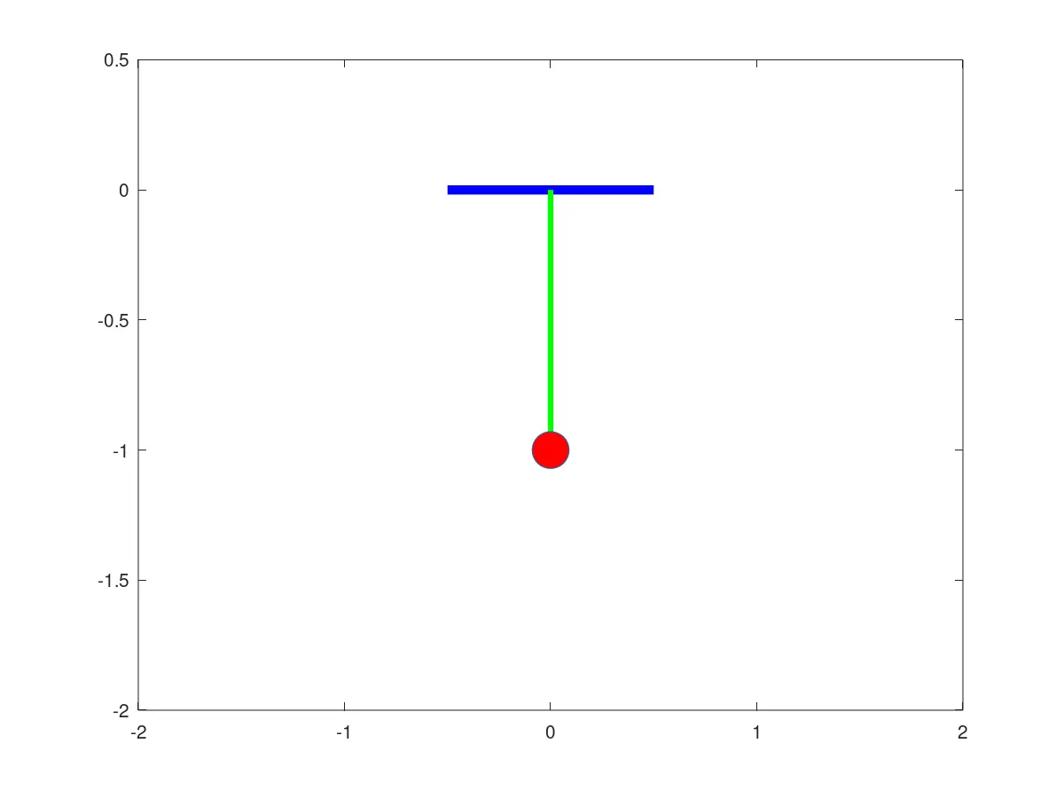
Q1. Write a program in MatlabOctave that will simulate the pendulum motion, just like the one shown in the start of this challenge.

use,

L=1 metre,

m=1 kg,

b=0.05.

g=9.81 m/s2.

Simulate the mtion between 0-20 sec, for angular displacement=0,angular velocity=3 rad/sec2 at time t=0.

1. You have to upload the animation on Youtube and paste the link to your answer.

2. Upload the code using "INSERT SAMPLE CODE" option and then post screenshot of the plots generated.

Ans:

The given equation is:

`(d^2 theta)/dt^2 + b/m((d theta)/dt) + g/l(sin theta)=0`

In order to solve the equation, certain assumptions are made which are :

`theta = theta1`

`(d theta)/dt =(d theta1)/dt= theta2`

Now,

`(d theta2)/dt + b/m (theta2) +g/l sintheta1=0`

`(d theta 2)/dt= -b/m(theta 2) -g/l sintheta1`

The function called in the main program is :

function[del_theta] = odefun_of_pendulum(y,t)
g=9.81;
l=1;
b=0.05;
m=1;
del_theta = zeros(2,1);
%velocity
del_theta(1) = y(2);
%acceleration
del_theta(2) = -0.05*y(2) - 9.81*sin(y(1));
end

The main function is:

close all
clear all
clc

t_span= linspace(0,20,400);
y_initial= [0 3]
%lsode command is udsed to solve the ode and returns the value of y.
[y] = lsode('odefun_of_pendulum',y_initial,t_span);
%graph 1 between t and y i.e time and angular position
figure(1);
plot(t_span,y(:,1),'b','linewidth',2)
hold on
%graph 2 between time and angular velocity
plot(t_span,y(:,2),'r','linewidth',2)
xlabel('time')
ylabel('dispplacement,velocity')
figure(2);
%graph 3 between angular position and angular velocity
plot(y(:,1),y(:,2),'g','linewidth',2)
xlabel('angular position')
ylabel('angular velocity')
%the for-loop for different postions of the pendulum 
figure(3);
ct=1;
for i=1:length(y(:,1))
x_0=0;
y_0=0;
x_1= 1*sin(y(i,1));
y_1= -1*cos(y(i,1));
plot([-0.5 0.5],[0 0],'b','linewidth', 5)
hold on
plot([0 x_1],[0 y_1],'linewidth',3,'g')
hold on
plot(x_1,y_1,'marker','o', 'markersize', 20, 'markerfacecolor', 'r')
axis([-2,2,-2,0.5])
hold off
pause(0.001);
%creating GIF file
% "sprintf" command is used to capture each frame of the pendulum.
videofile=sprintf("simple_pendulum%05d.png",ct); 
saveas(gca,videofile)
pause(0.03)
ct=ct+1;
end

Here we can see that the ''sprintf" command is used which is used to capture each 400 cases of the pendulum.

To stitch all the 400 cases into a single video, Magick software is used. After installing, the following commands are used:

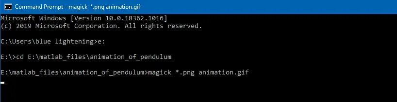
First using 'cd' command, set the location where all the .png files are saved.

Then using magick command and selecting all .png files a .gif file is formed named animation.gif.

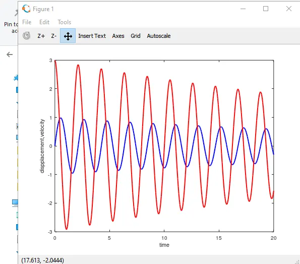
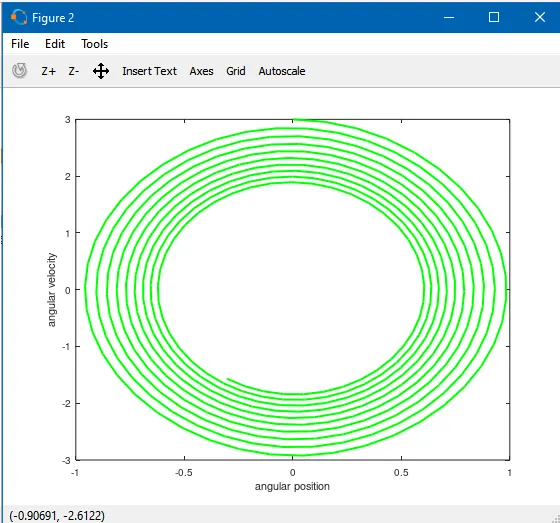
After running the above program, following results are obtained:

1. Plot 1- time vs displacement, velocity

2. Plot 2-

3. Plot 3- pendulum animation/gif

https://youtu.be/ZOnKmrGjTRI