Solving Steady and Transient State 2D Heat Conduction Equation
Objective:
- To find the solution for the steady and transient state 2D heat condution equation using various iterative methods and explicit method. The equations and conditions are:
- Steady State Heat Conduction Equation:
- `(del^2T)/(delx^2)+(del^2T)/(dely^2)=0`
- Transient/Unsteady State Heat Conduction Equation:
- `(delT)/(delt)-alpha*((del^2T)/(delx^2)+(del^2T)/(dely^2))=0`
- Here, T-Temperature in K, x,y-Spacial variables, t-Time in s, `alpha-`Thermal Diffusivity in `m^2"/"s`
- Boundary Conditions:
- Top Boundary: 600K
- Bottom Boundary: 900K
- Left Boundary: 400K
- Right Boundary: 800K
- Plate Dimensions: 1m X 1m
- Time step, dt= 1e-4s
- Thermal Diffusivity,`alpha`=1.4 `m^2"/"s`
- Tolerance(for iterative solvers)=1e-4
- Steady State Heat Conduction Equation:
Main Program:
clear all
close all
clc

%Inputs
nx=10;
ny=10;
x=linspace(0,1,nx);
y=linspace(0,1,ny);
dx=x(2)-x(1);
dy=y(2)-y(1);
tol=1e-4;
error=9e9;
%Initialising
for j=1:ny
    for i=1:nx
        T(j,i)=300;
    end
end
%Boundary Conditions
T(1,:)=600;     %Top
T(ny,:)=900;    %Bottom
T(:,1)=400;     %Left
T(:,nx)=800;    %Right
T(1,1)=500;     %Top-Left Corner
T(ny,1)=650;    %Bottom-Left Corner
T(1,nx)=700;    %Top-Right Corner
T(ny,nx)=850;   %Bottom-Right Corner

%Solving the equations
%Steady State Equation d^2T/dx^2 + d^2T/dy^2 = 0
%Jacobi method
    T_Jacobi=Jacobi_Sol_St(T,dx,dy,nx,ny,tol,error,x,y);

%Gauss Seidel method
    T_Gauss_Seidel=GS_Sol_St(T,dx,dy,nx,ny,tol,error,x,y);

%Successive Over Relaxation method
    T_Successive_Over_Relaxation=SOR_Sol_St(T,dx,dy,nx,ny,tol,error,x,y);

%Transient State Equation dT/dt - a*(d^2T/dx^2 + d^2T/dy^2)=0
%Explicit method
    T_Explicit_Transient_Final=Explicit_Sol_Tr(T,dx,dy,nx,ny,x,y);

%Jacobi method
    T_Jacobi_Transient_Final=Jacobi_Sol_Tr(T,dx,dy,nx,ny,tol,error,x,y);

%Gauss Seidel method
    T_Gauss_Seidel_Transient_Final=GS_Sol_Tr(T,dx,dy,nx,ny,tol,error,x,y);

%Successive Over Relaxation method
     T_Successive_Over_Relaxation_Transient_Final=SOR_Sol_Tr(T,dx,dy,nx,ny,tol,error,x,y);
Function #1: Jacobi_Sol_St(T,dx,dy,nx,ny,tol,error,x,y):
function out=Jacobi_Sol_St(T,dx,dy,nx,ny,tol,error,x,y)
k=2*(dx^2+dy^2)/(dx^2*dy^2);
Told=T;
while(error>tol)
    for j=2:ny-1
        for i=2:nx-1
            T(j,i)=((1/k)*(Told(j,i-1)+Told(j,i+1))/dx^2)+((1/k)*(Told(j-1,i)+Told(j+1,i))/dy^2);
        end
    end
    error=max(max(abs((Told-T))));
    Told=T;
end
figure(1)
contourf(x,y,T,'ShowText','on')
colormap(jet)
colorbar()
hold on
set(gca,'YDIR','reverse')
xlabel('X')
ylabel('Y')
title_text=sprintf('Steady State Jacobi');
title(title_text)
hold off
out=T;
end
Function #2: GS_Sol_St(T,dx,dy,nx,ny,tol,error,x,y):
function out=GS_Sol_St(T,dx,dy,nx,ny,tol,error,x,y)
k=2*(dx^2+dy^2)/(dx^2*dy^2);
Told=T;
while(error>tol)
    for j=2:ny-1
        for i=2:nx-1
            T(j,i)=((1/k)*(T(j,i-1)+Told(j,i+1))/dx^2)+((1/k)*(T(j-1,i)+Told(j+1,i))/dy^2);
        end
    end
    error=max(max(abs((Told-T))));
    Told=T;
end
figure(2)
contourf(x,y,T,'ShowText','on')
colormap(jet)
colorbar()
hold on
set(gca,'YDIR','reverse')
xlabel('X')
ylabel('Y')
title_text=sprintf('Steady State Gauss Seidel');
title(title_text)
hold off
out=T;
end
Function #3: SOR_Sol_St(T,dx,dy,nx,ny,tol,error,x,y):
function out=SOR_Sol_St(T,dx,dy,nx,ny,tol,error,x,y)
k=2*(dx^2+dy^2)/(dx^2*dy^2);
w=1.1;  %Relaxation factor
Told=T;
T_GS=T;
while(error>tol)
    for j=2:ny-1
        for i=2:nx-1
            T_GS(j,i)=((1/k)*(T_GS(j,i-1)+Told(j,i+1))/dx^2)+((1/k)*(T_GS(j-1,i)+Told(j+1,i))/dy^2);
            T(j,i)=((1-w)*Told(j,i))+(w*T_GS(j,i));
        end
    end
    error=max(max(abs((Told-T))));
    Told=T;
end
figure(3)
contourf(x,y,T,'ShowText','on')
colormap(jet)
colorbar()
hold on
set(gca,'YDIR','reverse')
xlabel('X')
ylabel('Y')
title_text=sprintf('Steady State Successive Over Relaxation');
title(title_text)
hold off
out=T;
end
Function #4: Explicit_Sol_Tr(T,dx,dy,nx,ny,x,y):
function out=Explicit_Sol_Tr(T,dx,dy,nx,ny,x,y)
a=1.4; %Thermal Diffusivity
dt=1e-4;
Told=T;
k1=a*dt/dx^2;
k2=a*dt/dy^2;
for nt=1:1400
    for j=2:ny-1
        for i=2:nx-1
            T(j,i)=Told(j,i)+k1*(Told(j,i-1)-2*(Told(j,i))+Told(j,i+1))+k2*(Told(j-1,i)-2*(Told(j,i))+Told(j+1,i));
        end
    end
    Told=T;
end
figure(4)
contourf(x,y,T,'ShowText','on')
colormap(jet)
colorbar()
hold on
set(gca,'YDIR','reverse')
xlabel('X')
ylabel('Y')
title_text=sprintf('Transient State Explicit');
title(title_text)
hold off
out=T;
end
Function #5: Jacobi_Sol_Tr(T,dx,dy,nx,ny,tol,error,x,y):
function out=Jacobi_Sol_Tr(T,dx,dy,nx,ny,tol,error,x,y)
a=1.4; %Thermal Diffusivity
dt=1e-4;
Told=T;
T_prev_dt=T;
k1=a*dt/dx^2;
k2=a*dt/dy^2;
term1=1/(1+(2*k1)+(2*k2));
term2=k1*term1;
term3=k2*term1;
for nt=1:1400
    error=9e9;
    while(error>tol)
        for j=2:ny-1
            for i=2:nx-1
                H=(Told(j,i-1)+Told(j,i+1));
                V=(Told(j-1,i)+Told(j+1,i));
                T(j,i)=(term1*T_prev_dt(j,i))+(term2*H)+(term3*V);
            end
        end
        error=max(max(abs((Told-T))));
        Told=T;
    end
    T_prev_dt=T;
end
figure(5)
contourf(x,y,T,'ShowText','on')
colormap(jet)
colorbar()
hold on
set(gca,'YDIR','reverse')
xlabel('X')
ylabel('Y')
title_text=sprintf('Transient State Jacobi');
title(title_text)
hold off
out=T;
end
Function #6: GS_Sol_Tr(T,dx,dy,nx,ny,tol,error,x,y):
function out=GS_Sol_Tr(T,dx,dy,nx,ny,tol,error,x,y)
a=1.4; %Thermal Diffusivity
dt=1e-4;
Told=T;
T_prev_dt=T;
k1=a*dt/dx^2;
k2=a*dt/dy^2;
term1=(1+(2*k1)+(2*k2))^-1;
term2=k1*term1;
term3=k2*term1;
for nt=1:1400
    error=9e9;
    while(error>tol)
        for j=2:ny-1
            for i=2:nx-1
                H=(T(j,i-1)+Told(j,i+1));
                V=(T(j-1,i)+Told(j+1,i));
                T(j,i)=(term1*T_prev_dt(j,i))+(term2*H)+(term3*V);
            end
        end
        error=max(max(abs((Told-T))));
        Told=T;
    end
    T_prev_dt=T;
end
figure(6)
contourf(x,y,T,'ShowText','on')
colormap(jet)
colorbar()
hold on
set(gca,'YDIR','reverse')
xlabel('X')
ylabel('Y')
title_text=sprintf('Transient State Gauss Seidel');
title(title_text)
hold off
out=T;
end
Function #7: SOR_Sol_Tr(T,dx,dy,nx,ny,tol,error,x,y):
function out=SOR_Sol_Tr(T,dx,dy,nx,ny,tol,error,x,y)
a=1.4; %Thermal Diffusivity
w=1.1; %Relaxation factor
dt=1e-4;
Told=T;
T_prev_dt=T;
T_GS=T;
k1=a*dt/dx^2;
k2=a*dt/dy^2;
term1=1/(1+(2*k1)+(2*k2));
term2=k1*term1;
term3=k2*term1;
for nt=1:1400
    error=9e9;
    while(error>tol)
        for j=2:ny-1
            for i=2:nx-1
                H=(T_GS(j,i-1)+Told(j,i+1));
                V=(T_GS(j-1,i)+Told(j+1,i));
                T_GS(j,i)=(term1*T_prev_dt(j,i))+(term2*H)+(term3*V);
                T(j,i)=(1-w)*Told(j,i)+w*T_GS(j,i);
            end
        end
        error=max(max(abs((Told-T))));
        Told=T;
    end
    T_prev_dt=T;
end
figure(7)
contourf(x,y,T,'ShowText','on')
colormap(jet)
colorbar()
hold on
set(gca,'YDIR','reverse')
xlabel('X')
ylabel('Y')
title_text=sprintf('Transient State Successive Over Relaxation');
title(title_text)
hold off
out=T;
end
Explanation:
- The 'close all', 'clear all', and 'clc' commands are used to close and clear the existing outputs and variables used.
- Then inputs such as the number of nodes along 'x' and 'y' direction, 'nx' and 'ny'; the nodal values along 'x' and 'y' direction, array 'x' and 'y' are given; subsequently the nodal lengths, 'dx' and 'dy' are calculated. Then the tolerance value and error are provided as per the given values.
- Now, the temperature is initialised for the entire domain of the plate. As it is a plate, two 'for' loops are used to accomplish the same.
- As provided, the boundary conditions are applied for all the four sides and the corners(average of the adjacent values)
- Now that the initial values and boundary conditions are specified, the functions to solve the equations are called one by one. The function explanations are as follows:
- Firstly, the steady state equation is solved using the three iterative methods, Jacobi, Gauss Seidel and Successive Over Relaxation(SOR) by calling the respective function. Now, for solving the steady state equation using Jacobi method, the function Jacobi_Sol_St(T,dx,dy,nx,ny,tol,error,x,y) is used.
- The function takes T,dx,dy,nx,ny,tol,error,x,y as input and returns the final 'T' value as the output.
- The Steady State heat conduction equation is `(d^2T)/dx^2 + (d^2T)/dy^2 = 0` and it is discretized using central difference scheme as the equation is similar to elliptical form & is rewritten as:
- `T(j,i)=((1/k)*(Told(j,i-1)+Told(j,i+1))/dx^2)+((1/k)*(Told(j-1,i)+Told(j+1,i))/dy^2)`
- where `k=2*(dx^2+dy^2)/(dx^2*dy^2)`, 'Told' values are the values from previous iteration, since it's Jacobi method the old iteration values are used to find the value for current iteration. Note: The info from all sides are taken as it is a central difference scheme. Here,`(Told(j,i-1),Told(j,i+1)` represent the left and right values w.r.t. to point at which the temperature value is calculated. Similarly, `Told(j-1,i),Told(j+1,i)` represent the top and bottom values.
- Having the discretized equation, the value at each point is found using two 'for' loops. Then, the error is computed comparing with the previous iteration values.
- In order to facilitate the passage of the next iteration, the 'Told' value is updated with the current value. And the error is compared with the tolerance value specified to check for convergence of the solution using the outermost 'while' loop.
- After the convergence is reached(i.e., the error value becomes less than the tolerance value), the temperature value is plotted for the entire domain using 'contourf' function. The 'ShowText' attribute is used to display the temperature value at various locations of the plot so as to give clarity.
- The 'colormap()' function is used to specify which color pallet to be employed and the 'colorbar()' function to display the color bar as legend to the plot.
- As Matlab computes the values from top to botom and left to right, the first value is in the top-left corner, but contourf plots it in upside down fashion, so the Y axis is inverted using 'set()' function.
- Then, the 'xlabel' and 'ylabel' commands are used to define the x-axis and y-axis.
- To add heading to the plot, the 'title()' function is used.
- Similarly, for solving the steady state equation using Gauss Seidel and Successive Over Relaxation methods, the functions GS_Sol_St(T,dx,dy,nx,ny,tol,error,x,y) and SOR_Sol_St(T,dx,dy,nx,ny,tol,error,x,y) are used.
- Only the discretized equation varies in each case. The equation for Gauss Seidel method is:
- `T(j,i)=((1/k)*(T(j,i-1)+Told(j,i+1))/dx^2)+((1/k)*(T(j-1,i)+Told(j+1,i))/dy^2)`
- where `k=2*(dx^2+dy^2)/(dx^2*dy^2)`, 'Told' values are the values from previous iteration and 'T' values are the values from current iteration, which are already computed before reaching the current point. It's Gauss Seidel method so both the old iteration values and the current iteration values, which are computed before reaching the current point(i.e., the left point and the top point) are used to find the value for current iteration.
- The value for Successive Over Relaxation method is found, in two steps, by finding the value for gauss seidel method in that iteration and then finding the difference between the previous iteration & current iteration value and amplifying this difference by a relaxation factor, 'w'. (Note: This helps in reducing the number of iterations and the computation time).
- `T_(GS)(j,i)=((1/k)*(T_(GS)(j,i-1)+Told(j,i+1))/dx^2)+((1/k)*(T_(GS)(j-1,i)+Told(j+1,i))/dy^2)`
- `T(j,i)=Told(j,i)+w*(T_(GS)(j,i)-Told(j,i))`
- `=>T(j,i)=((1-w)*Told(j,i))+(w*T_(GS)(j,i))`
- As the steady state equation has been solved using all the implicit methods, now the transient equation is solved. To start with, it's solved using explicit method by calling Explicit_Sol_Tr(T,dx,dy,nx,ny,x,y).
- Firstly, the transient state equation is `(dT)/dt - a*((d^2T)/dx^2 + (d^2T)/dy^2)=0`
- It is discretized using time marching solution method for the first term and central difference scheme for the second part as they resemble hyperbolic equation and elliptical equation respectively. The discretized equation for explicit method is as follows:
- `T(j,i)=Told(j,i)+k1*(Told(j,i-1)-2*Told(j,i)+Told(j,i+1))+k2*(Told(j-1,i)-2*Told(j,i)+Told(j+1,i))`
- where `k1=a*dt/dx^2; k2=a*dt/dy^2`
- Note: As it is explicit method the respective values in the previous time-step are used to find the values in current time-step, so no iterative solver required.
- Now, to code it in Matlab, the outer-most loop is taken as time loop as it is transient and then the temperature value at each point is found using two for loops by using the above equation. (Note: There is no need for convergence loop as it isn't implicit method, where error is captured and convergence is tested, only time loop is taken)
- Then similar to the previous functions, the final value is plotted using 'contourf()' function and the required attributes and other fromatting are carried out.
- Next, the transient equation is solved using the three implicit methods one by one. At first, it is solved using Jacobi method. The function Jacobi_Sol_Tr(T,dx,dy,nx,ny,tol,error,x,y) is used to perform the same, the explanation is as follows.
- The constant values are first initialised and then the algorithm to solve the equation starts.
- Here , a loop to regulate the time-step, then one to check for convergence and two loops for spacial variables are employed as it is an implicit method.
- The discretized equation is:
- `=>T(j,i)=(1/(1+(2*k1)+(2*k2))*T_(prev_dt)(j,i))+(k1*1/(1+(2*k1)+(2*k2))*(Told(j,i-1)+Told(j,i+1)))+(k2*1/(1+(2*k1)+(2*k2))*(Told(j-1,i)+Told(j+1,i)))`
- As it is implicit, the equation contains current time-step unknowns to find the value at a particular point. So, it's solved in iterative method. Hence the above equation is deduced after rearranging the like terms.
- As the equation is complex, it's computed in three steps as follows:
- `H=(Told(j,i-1)+Told(j,i+1)); V=(Told(j-1,i)+Told(j+1,i));`
- `=>T(j,i)=(term1*T_(prev_dt)(j,i))+(term2*H)+(term3*V)`
- where `term1=1/(1+(2*k1)+(2*k2)); term2=k1*term1; term3=k2*term1;`
- `k1=a*dt/dx^2; k2=a*dt/dy^2;`
- (Note: Here, `T_(prev_dt)`is the value in the previous time-step, where as `Told` is the value in the previous iteration in the current time-step)
- The value is computed for each point and after computing it for the entire domain, it is checked for convergence by finding the error and then comparing it with tolerance. Once it converges, the `T_(prev_dt)` is updated with the current value and the loop goes to the next time-step.
- Finally, after finding the value for the last time-step, it is plotted using 'contourf()' as usual.
- Similarly, the equation is solved using Gauss Seidel and Successive Over Relaxation methods using the functions GS_Sol_Tr(T,dx,dy,nx,ny,tol,error,x,y) and SOR_Sol_Tr(T,dx,dy,nx,ny,tol,error,x,y) respectively.
- Only the equation alone changes for each of the method. For Gauss Seidel method the equation is:
- `H=(T(j,i-1)+Told(j,i+1));`
- `V=(T(j-1,i)+Told(j+1,i));`
- `T(j,i)=(term1*T_((prev)_(dt))(j,i))+(term2*H)+(term3*V);`
- Here, as it is Gauss Seidel method, the current iteration values which are calculated before the current point are used in the equation and the rest of the values are old iteration values.
- The equation for Successive Over Relaxation method is:
- `T(j,i)=Told(j,i)+w*(T_(GS)(j,i)-Told(j,i))`
- `=>T(j,i)=(1-w)*Told(j,i)+w*T_(GS)(j,i)`
- Here, w-Relaxation factor
- `T_(GS)(j,i)=(term1*T_((prev)_(dt))(j,i))+(term2*H)+(term3*V);`
- `term1=1/(1+(2*k1)+(2*k2)); term2=k1*term1; term3=k2*term1;`
- `H=(T_(GS)(j,i-1)+Told(j,i+1));``V=(T_(GS)(j-1,i)+Told(j+1,i));`
- For SOR method, as it amplifies the difference between previous iteration values and current iteration values calculated using Gauss Seidel method, it is accomplished in four steps as shown above.
- Firstly, the steady state equation is solved using the three iterative methods, Jacobi, Gauss Seidel and Successive Over Relaxation(SOR) by calling the respective function. Now, for solving the steady state equation using Jacobi method, the function Jacobi_Sol_St(T,dx,dy,nx,ny,tol,error,x,y) is used.
- As all the required methods have been used to find the solution and plot the same, the main code is complete.
Output Explanation:
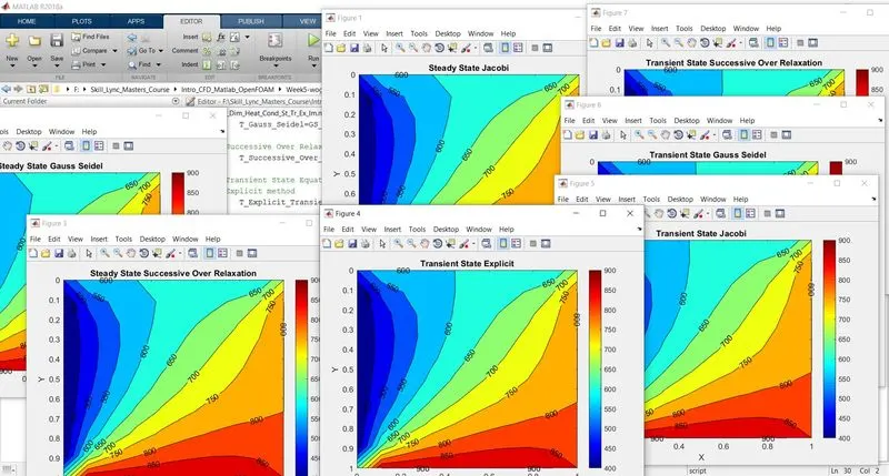
- Output Screen:
- Observation & Inference:
- The graphs and values are displayed, which shows that the code has executed successfully without any errors.
- All the seven plots, three plots for steady state solution and four for transient state, are generated.
- Plots Comparison:
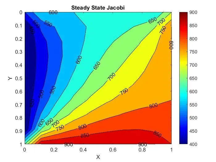
- Steady State Jacobi:
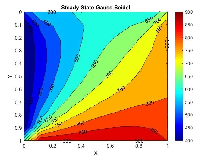
- Steady State Gauss Seidel:
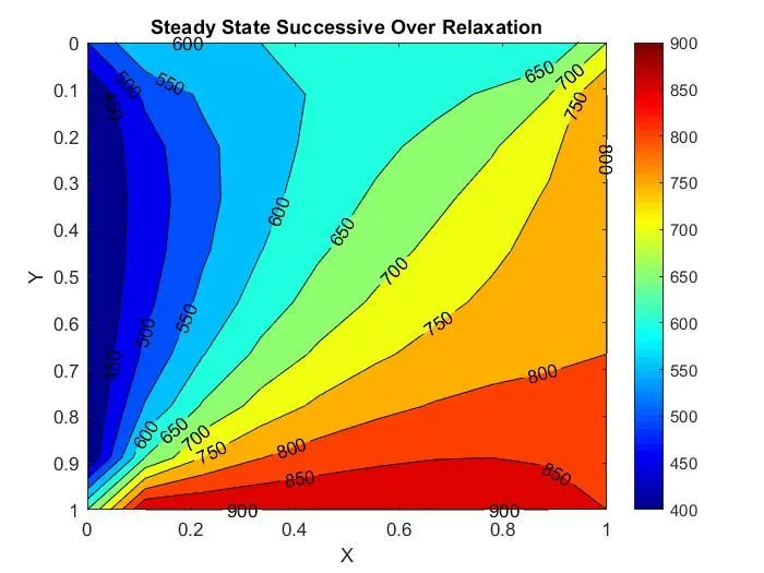
- Steady State Successive Over Relaxation:
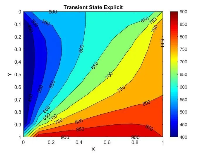
- Transient State Explicit:
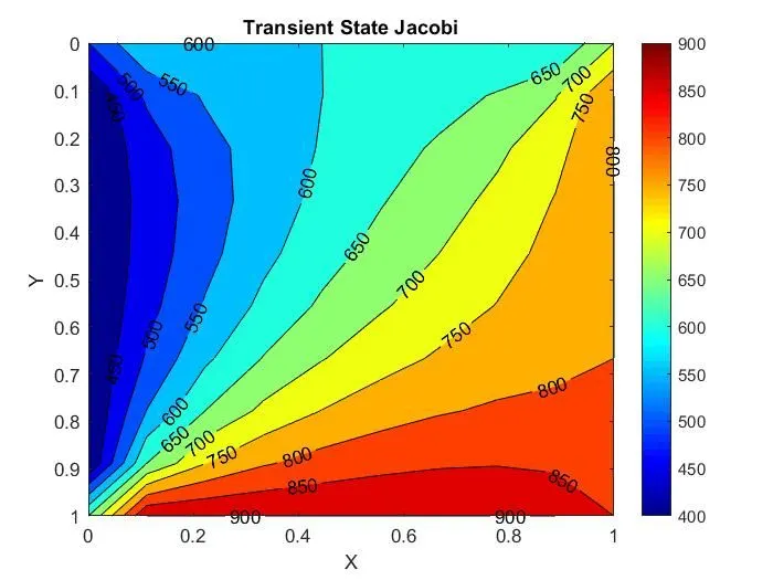
- Transient State Jacobi:
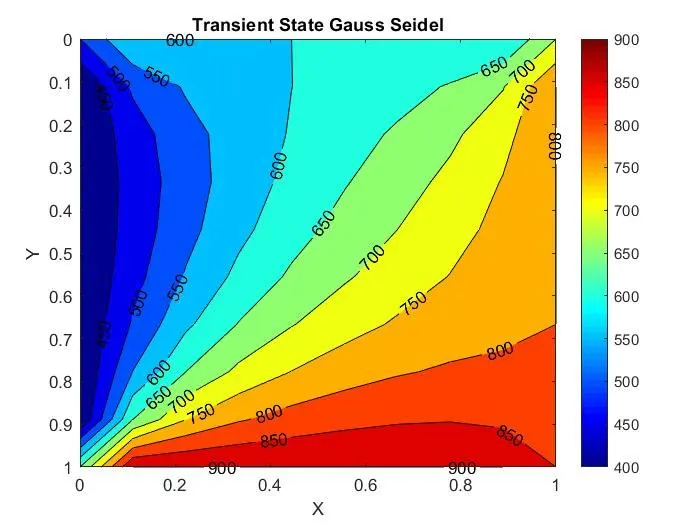
- Transient State Gauss Seidel:
- Transient State Successive Over Relaxation:
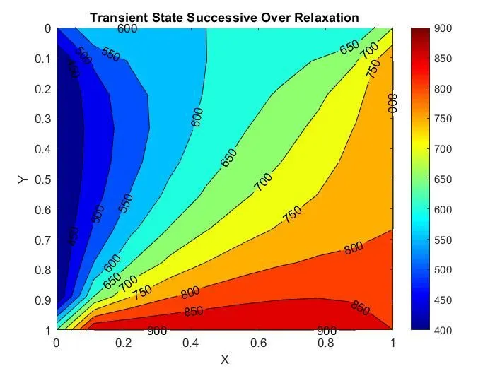
- Observation and Inference:
- The variation of temperature along the square plate for steady and transient condition is depicted in the above plots. Also, each represent the method from which the solution is arrived.
- The temperature is the highest at the bottom(900K) and lowest at the left(400K) as initialised. The temperature of the entire plate increases from the initial value as the heat conducts from high temperature region to low temperature region.
- The transient simulation is run for 1400 time-steps and the temperature distribution after this is plotted, which is similar to that of the steady state simulation.
- Steady State Jacobi:
Result:
- The 2D heat conduction equation has been solved for both steady and transient states using various implicit methods and explicit method(transient state).
- The resultant contours have been plotted and analysed.