Solving second order Ordinary Differential Equations (ODEs) of a Simple Pendulum using Python

Objective:

Write a program to solve an ODE which represents the equation of motion of a simple pendulum with damping and animate a simple pendulum in motion.

Simple Pendulum:

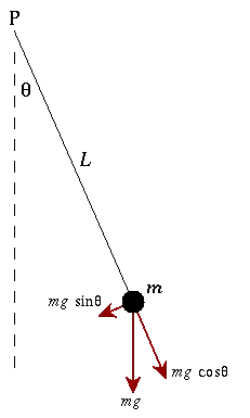
A simple pendulum consists of a ball (point-mass) m hanging from a (massless) string of length L and fixed at a pivot point P. When displaced to an initial angle and released, the pendulum will swing back and forth with periodic motion. By applying Newton's secont law for rotational systems, the equation of motion for the pendulum may be obtained

`tau=Ialpha = -mgsinthetaL=mL^2(d^2theta)/dt`

and rearranged as

`(d^2theta)/dt^2+g/L sintheta=0`

and if a damper is introduced in the system the above equation becomes

`(d^2theta)/dt^2+b/m (d theta)/dt +g/L sintheta=0`

In the above equation,

g = gravity in m/s^2,

L = length of the pendulum in m,

m = mass of the ball in kg,

b=damping coefficient.

Governing Equations:

To solve the above equation in Python, we need to transform the given second order ODE into first order ODE:

suppose `theta = theta_1`

`(d theta)/dt = (d theta_1)/dt = theta_2` .(I)

`(d^2 theta)/dt^2 = (d^2 theta_1)/dt^2 = d/dt((d theta_1)/dt) = d/dt(theta_2)` .(II)

ODE: `(d^2theta)/dt^2+b/m (d theta)/dt +g/L sintheta=0`

Replacing `theta with theta_1`

`(d^2theta_1)/dt^2+b/m (d theta_1)/dt +g/L sintheta_1=0`

by replacing the values with equation II

`(d theta_2)/dt+b/m theta_2 +g/L sintheta_1=0`

`(d theta_2)/dt = -b/m theta_2 -g/L sintheta_1`

so we get two first order ODE's, `(d theta_1)/dt = theta_2`,`(d theta_2)/dt = -b/m theta_2 -g/L sintheta_1`

Python Code:

"""
Simple Pendulum animation and ODE solution by Giridhar
"""
import math
import matplotlib.pyplot as plt
import numpy as np
from scipy.integrate import odeint

# function that returns dz/dt
def model(theta,t,b,g,l,m):
	theta1 = theta[0]
	theta2 = theta[1]
	dtheta1_dt = theta2
	dtheta2_dt = -(b/m)*theta2-(g/l)*math.sin(theta1)
	dtheta_dt = [dtheta1_dt,dtheta2_dt]
	return dtheta_dt
# Inputs 
# damping coefficient
b = 0.05
# gravity(m/s^2)
g = 9.81  
# length of the pendulum (m)                                                               
l = 1  
# mass of ball (kg)                                                                  
m = 1      

# Initial Conditions
theta_0 = [0,3] 

# time points
t = np.linspace(0,20,150)

# ode solution
theta = odeint(model,theta_0,t,args = (b,g,l,m))

# plotting the results
plt.plot(t,theta[:,0],'b-',Label = r'$frac{dtheta1}{dt}=theta2$(Displacement)')
plt.plot(t,theta[:,1],'r--',Label = r'$frac{dtheta2}{dt}=-frac{b}{m}theta2-frac{g}{l}sintheta1$(Velocity)')
plt.xlabel('Time (s)')
plt.ylabel('Plot')
plt.title('Harmonic motion of a Pendulum_Damped')
plt.legend(loc='best')
plt.savefig('Pendulum_Damped')
plt.show()

# Animation of Pendulum motion 

ct =1
tmp = theta[:,0]
for i in tmp:
	x_start = 0                                                           
	y_start = 0
	x_end =  l*math.sin(i)                                          
	y_end = -l*math.cos(i)

	filename = str(ct) + '.png'
	ct = ct + 1
	
	plt.figure()
	# string
	plt.plot([x_start,x_end],[y_start,y_end],linewidth=3)
	# pendulum ball
	plt.plot(x_end,y_end,'o',markersize=15,color='y')
	# support
	plt.plot([-1.25,1.25],[0,0],linewidth=5,color='k')
	plt.plot([0,0],[0,-1.5],'--',color='r')
	plt.xlim([-1.25,1.25])
	plt.ylim([-1.5,1.5])
	plt.title('Animation of a Pendulum')
	plt.savefig(filename)

Plot:

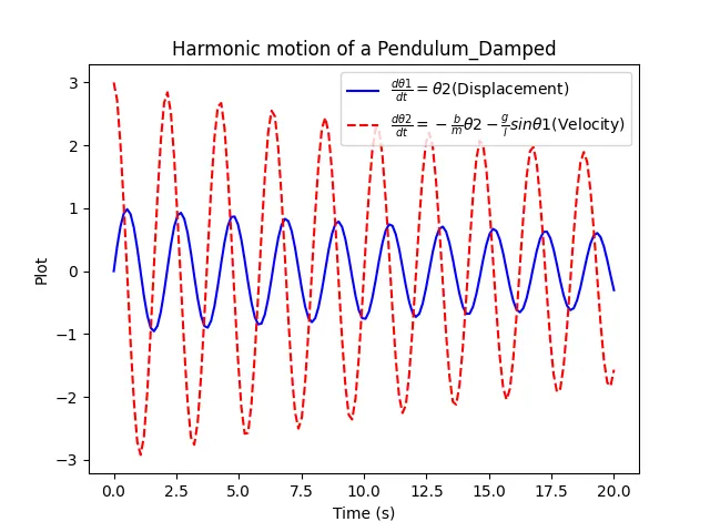
The above plot of angular displacement and angular velocity shows the pendulum's motion to be gradually decreasing. This is due to the damping effect which decreases the amplitude and the velocity of motion.

Pendulum Motion Animation:

Errors:

• The first 2 errors are related to version 3.3 and did not cause any trouble to coding and output.
• The third error is regarding the number of figures saved. As there are 150 figures generated, the software is warning about consuming too much memory to create the same.

Python Code Explanation:

• Math module is imported as the code contains mathematical calculations.
• matplotlib.pyplot as plt is imported as we need plots from the calculations performed.
• numpy is imported for arrays.
• odeint is imported from scipy.integrate for solving ODE.
• A function is defined with undefined variables of theta1 and theta 2 and will be defined outside of the function.
• The value of dtheta_dt is returned back to the function.
• Inputs such as b,g,l,m are provided according to function.
• An array of theta was created to define Angular displacement and Angular velocity.
• An array of a time points was created to store 150 equally spaced intervals between 0 to 20 seconds.
• The function is called to solve ODE and odeint command is used as a prefix.
• plt.plot command is used to plot the graph of variation of angular displacement and angular velocity wrt time.
• plt._label is used for assingning lables to the graph, plt.title is used for the title of the graph.
• The plot is saved using plt.savefig command and shown using plt.show command.

Simple Pendulum Animation:

• ct=1 is assigned before for loop and ct= ct+1 inside the loop, so that each figure is saved with the name starting with 1 and incremented by 1.
• A for loop is used to give the values of angular position and is stored in tmp and iterated.
• plt.plot is used to plot string, ball, the center line (axis) and support etc required for animation.
• plt._lim command is used to define limits in coordinates for the whole graph.
• The plot is saved using plt.savefig command.
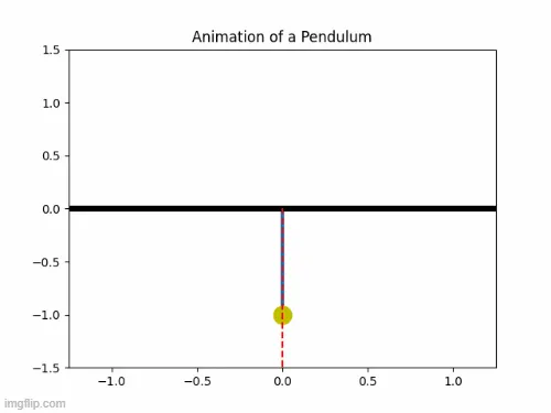
• These .png files are converted into a gif file using the imgflip.com. We can also do it using the cygwin and imagemagick softwares together.

Conclusion:

A program in Python is created and succesfully executed to solve Ordinary Differential Equations of a damped pendulum and animated a simple pendulum in motion.