Solving 2D heat conduction equation using various iterative solvers.
Aim :
To conduct the steady state and transient state analysis by solving the 2D heat conduction equation using various iterative solvers.
Objectives:
- To solve the 2D heat conduction equation by finite difference method.
- To made a steady state analysis by solving the 2D heat conduction equation by using jacobi, gauss seidel and successive over relaxation solvers.
- To made the transient state analysis for both explicit and implicit schemes.
- To analyse the results for the three types of iterative solvers applied to explicit and implicit schemes separately.
- To analyse the optimum solver by taking the number of iteration and time factors in account.
Heat conduction:
The thermal conduction or heat conduction is the phenomenon in which the internal energy is transfered within a body. This phenomenon is happening by the microscopic collisions or by the movement of electrons within the body. The thermal conduction takes place in all phases. This conduction is also defined by the term heat transfer. The heat transfer carried out the conduction process from one surface with higher temperature to the another surface with lower temperature in a body. There are three modes of heat transfer based on the medium. The conduction heat transfer occurs in between the solids. The convection heat transfer occurs between the solid to liquid. THe radiation heat transfer happens without any medium. The heat conduction takes place in four various states.
a) Steady-state heat conduction:
The steady state heat conduction is a type in which the temperature difference is constant within the body. In the steady state heat conduction the spatial distribution of temperature does not change any further in the conducting object. The total heat that entering into the body from any region will be equal to the total heat that coming out from the body.
b) Transient heat conduction:
The transient heat conduction is also defined as unsteady-state heat conduction. It is a mode of heat conduction in which the temperature changes in time at any place within the body over a period of time. It is also defined as the time dependent state of heat conduction. The analysis of transient heat conduction is bit difficult when compared with steady-state heat conduction.
Governing equation of 2D heat conduction:
The governing equation provide the nature of the conduction phenomenon. The heat equation which represent the temperature change with respect to time on all the three axes are represented below,
`(delT)/(delt)=alpha*((del^2T)/(delx^2)+(del^2T)/(dely^2)+(del^2T)/(delz^2))`
where, T - Temperature,
`alpha`- Thermal diffusivity of the medium,
x,y,z - space coordinates,
t - time coordinate.
The heat equation is converted into the 2D heat conduction governing equation by considering the respective factors. The governing equation for the steady state heat conduction and transient state heat conduction is represent below,
1) For steady state heat conduction:
`((del^2T)/(delx^2)+(del^2T)/(dely^2))=0`
2) For transient state heat conduction:
`(delT)/(delt) = alpha.((del^2T)/(delx^2)+(del^2T)/(dely^2))`
These two governing equations are solved using the finite difference method.
Discretization:
The discretization is a process of converting a continuous big model or function into discrete or smaller nodes to analyse the nature or results in the domain accurately.
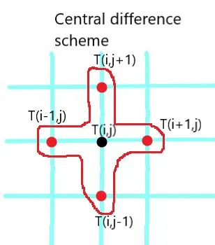
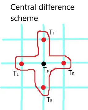
The finite difference method is used in which the central difference scheme is applied to discretize the governing equation for steady state and transient state heat conduction. The central difference scheme is a method of finding or simulating the centre point by taking the successive and precessive points. For 2D condition the points at left,right,top and bottom to the reference point is took in consider.
1) Steady-state heat conduction:
The governing equation for steady state heat conduction is,
`((del^2T)/(delx^2)+(del^2T)/(dely^2))=0`
By applying the central difference scheme in finite difference method,
`((T_(i-1,j)^n-2T_(i,j)^n+T_(i+1,j)^n)/(Deltax^2))+((T_(i,j-1)^n-2T_(i,j)^n+T_(i,j+1)^n)/(Deltay^2))=0`
By replacing the node points based on their position,
`T_(i-1,j)=T_L`
`T_(i,j)=T_P`
`T_(i+1,j)=T_R`
`T_(i,j-1)=T_B`
`T_(i,j+1)=T_T`
Note : This is for the easy representation of nodes in the equation.
`((T_(L)^n-2T_(P)^n+T_(R)^n)/(Deltax^2))+((T_(B)^n-2T_(P)^n+T_(T)^n)/(Deltay^2))=0`
By simplifying the above equation,
`T_(i,j)^n=(1/k)*((T_R^n+T_L^n)/(Deltax^2)+(T_T^n+T_B^n)/(Deltay^2))`
where, `k=2*((Deltax^2+Deltay^2)/(Deltax^2*Deltay^2))`
2) Transient-state heat conduction (Explicit):
The governing equation for the transient-state heat conduction is,
`(delT)/(delt) = alpha.((del^2T)/(delx^2)+(del^2T)/(dely^2))`
By discretizing the above equation using finite difference method under central difference scheme,
`(T_P^(n+1)-T_P^n)/(Deltat)=alpha.((T_L-2T_P+T_R)/(Deltax^2)+(T_T-2T_P+T_B)/(Deltay^2))^n`
=> `T_P^(n+1) - T_P^n= alpha.Deltat((T_L-2T_P+T_R)/(Deltax^2)+(T_T-2T_P+T_B)/(Deltay^2))^n`
By simplifying the above equation,
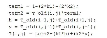
`T_P^(n+1)=T_P^n+k1(T_L-2T_P+T_R)^n+k2(T_T-2T_P+T_B)^n`
where, `k1=alpha((Deltat)/(Deltax^2))`
`k2=alpha((Deltat)/(Deltay^2))`
The term 'k' defined as the CFL numbers. k1-CFL number along x axis and k2-CFL number along y axis.
3) Transient-state heat conduction (Implicit):
The final discretized equation for the transient-state heat conduction (implicit) using FDM method is,
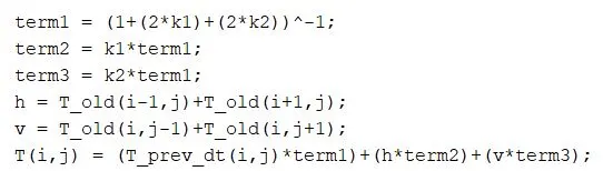
`T_P^(n+1)=(1/(1+2*k1+2*k2))(T_P^n+k1*(T_L+T_R)^(n+1)+k2*(T_T+T_B)^(n+1))`
Inputs and Boundary conditions:
- The domain is of unit length.
- The number of points along x-axis (nx) is equal to the number of points along y-axis (ny).
- The boundary conditions are,
1. Top Boundary = 600 K
2. Bottom Boundary = 900 K
3. Left Boundary = 400 K
4. Right Boundary = 800 K
- Absolute error or tolerance = 1e-4
- The steady state and transient state simulation should be done under jacobi,gauss seidel and successive over relaxation(SOR) solvers.
Iterative solvers:
1) Jacobi method:
The jacobi method is one of the iterative methods for solving governing equation. The discretized equation is solved by assuming some values for the intial solution. The solving process took place till the converged results are obtained. Once a final value is obtained in one iteration, the values are changed by the values obtained in the previous iteration.
For steady-state heat conduction:

For transient-state heat conduction(Explicit):
For transient-state heat conduction(Implicit):
2) Gauss seidel method:
The gauss seidel method is a type of iterative solver in which the values of the unknowns are assigned initially to get the intial solution as done in jacobi method. The main difference is once a value for an unknown is found, this value is used to get the another value in a same iteration under gauss seidel method. The jacobi method is done with a set of values for one complete iteration. There is not any updation of values occur in jacobi method.
For steady-state heat conduction:

For transient-state heat conduction(Explicit):
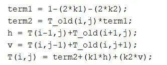
For transient-state heat conduction(Implicit):
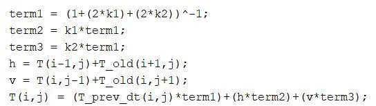
3) Successive Over Relaxation(SOR) method:
The successive over relaxation method is an effective iterative solver. The SOR method uses either the solution obtained from jacobi method or from gauss seidel method. In additional to it, the relaxation factor(`omega`) is took in consider in case of SOR method.
Generally, In SOR --> `T_(i,j)=(1-omega)T_(old)+omega*`(Final equation of either gauss seidel or jacobi method).
For steady-state heat conduction:

For transient-state heat conduction(Explicit):
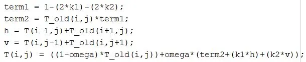
For transient-state heat conduction(Implicit):

Code:
1) Steady-state heat conduction:
clear all
close all
clc

%Steady-state heat conduction
%Input values
%length of domain
l = 1;

%Number of Grid points
nx = 40;
ny = nx;
x = linspace(0,l,nx);
y = linspace(0,l,ny);

dx = x(2) - x(1);
dy = y(2) - y(1);

%k value calculation
k = 2*((dx^2+dy^2)/(dx^2*dy^2));

%Error and tolerance value
error = 9e9;
tolerance = 1e-4;

%Omega value for SOR method
omega = 1.2;

%Boundary condition
T_top = 600;
T_bottom = 900;
T_left = 400;
T_right = 800;

T = ones(nx,ny);
T(1,:) = 600;
T(end,:) = 900;
T(:,1) = 400;
T(:,end) = 800;

%T old value
T_old = T;

%Type of iterative solver
Iterative_solver = 1;

%Jacobi method
tic
if Iterative_solver == 1

    jacobi_iter = 1;
    while (error > tolerance)
        for i = 2:nx-1
            for j = 2:ny-1

                term1 = (T_old(i+1,j)+T_old(i-1,j))/(dx^2);
                term2 = (T_old(i,j+1)+T_old(i,j-1))/(dy^2);
                T(i,j) = (term1+term2)/k;
            end
        end
        %Error value calculation
        error = max(max(abs(T_old-T)));

        %Updating T_old value
        T_old = T;

        %Incrementation
        jacobi_iter = jacobi_iter + 1;

    end
    time = toc;

    %Plotting
    figure(1)
    colormap(jet)
    contourf(x,y,T,'showText','on')
    title({['Steady state - jacobi method'];['Iteration : ',num2str(jacobi_iter)];['Time : ',num2str(time)]})
    xlabel('x-axis')
    ylabel('y-axis')
    set(gca,'Ydir','reverse')
    colorbar

end

%Gauss seidel method
tic
if Iterative_solver == 2

    GS_iter = 1;
    while (error > tolerance)
        for i = 2:nx-1
            for j = 2:ny-1

                term1 = (T_old(i+1,j)+T(i-1,j))/(dx^2);
                term2 = (T_old(i,j+1)+T(i,j-1))/(dy^2);
                T(i,j) = (term1+term2)/k;
            end
        end

        %Error value calculation
        error = max(max(abs(T_old-T)));

        %Updating T_old vlaue
        T_old = T;

        %Incrementation
        GS_iter = GS_iter + 1;

    end
    time = toc;

    %Plotting
    figure(1)
    colormap(jet)
    contourf(x,y,T,'showText','on')
    title({['Steady state - Gauss seidel method'];['Iteration : ',num2str(GS_iter)];['Time : ',num2str(time)]})
    xlabel('x-axis')
    ylabel('y-axis')
    set(gca,'Ydir','reverse')
    colorbar
end

%SOR method
tic
if Iterative_solver == 3

    SOR_iter = 1;
    while (error > tolerance)
        for i = 2:nx-1
            for j = 2:ny-1

                term1 = (T_old(i+1,j)+T(i-1,j))/(dx^2);
                term2 = (T_old(i,j+1)+T(i,j-1))/(dy^2);
                T(i,j) = ((1-omega)*T_old(i,j))+(omega*((term1+term2)/k));
            end
        end

        %Error value calculation
        error = max(max(abs(T_old-T)));

        %Updating T_old value
        T_old = T;

        %Incrementation
        SOR_iter = SOR_iter + 1;
    end
    time = toc;

    %Plotting
    figure(1)
    colormap(jet)
    contourf(x,y,T,'showText','on')
    title({['Steady state - SOR method'];['Iteration : ',num2str(SOR_iter)];['Time : ',num2str(time)]})
    xlabel('x-axis')
    ylabel('y-axis')
    set(gca,'Ydir','reverse')
    colorbar

end
Code explanation:
- The input values like length of the domain (l), nx and other values are assigned initially.
- From the input values, various terms such as dx,dy, and k are found.
- The boundary conditions are assigned both in values and position of it in grid.
- The iterative solver is choosed.
- 'If' loop is opened for the three different solvers separately.
- The space loops for two axes are opened before this the convergence loop is opened.
- Based on the selected iterative solver, the respective final equation for the solver is solved within these loops.
- After the space loop or before the end of convergence loop, the error value was found, T_old value gets updated and incrementation take place.
- Finally, after the end of convergence loop, plotting was made.
- "colormap(jet)" command represent the plot with an array of colors in which red,green and blue has a maximum intensity.
- "contourf" command is used to represent the 2D plot.
- The "set(gca,'Ydir','reverse')" command is used to reverse the y-axis and values to get the optimum view of plot.
2) Transient-state heat conduction(Explicit):
clear all
close all
clc

%Input values
%length of domain
l = 1;

%Number of Grid points
nx = 40;
ny = nx;
x = linspace(0,l,nx);
y = linspace(0,l,ny);

dx = x(2) - x(1);
dy = y(2) - y(1);

%Thermal diffusivity value (alpha)
alpha = 1.5;
dt = 0.0001;

%CFL numbers value calculation
k1 = alpha*(dt/(dx)^2);
k2 = alpha*(dt/(dy)^2);

%Relaxation factor value for SOR method
omega = 1.2;

%Boundary condition
T_top = 600;
T_bottom = 900;
T_left = 400;
T_right = 800;

T = ones(nx,ny);
T(1,:) = 600;
T(end,:) = 900;
T(:,1) = 400;
T(:,end) = 800;

%T old value
T_old = T;

%Type of iterative solver
Iterative_solver = 3;

%Time step
nt = 1500;

%Jacobi method
tic
if Iterative_solver == 1

   for k = 1:nt
        for i = 2:nx-1
            for j = 2:ny-1

                term1 = 1-(2*k1)-(2*k2);
                term2 = T_old(i,j)*term1;
                h = T_old(i-1,j)+T_old(i+1,j);
                v = T_old(i,j-1)+T_old(i,j+1);
                T(i,j) = term2+(k1*h)+(k2*v);
            end
        end
        %Updating T_old value
        T_old = T;

    end
    time = toc;

    %Plotting
    figure(1)
    colormap(jet)
    contourf(x,y,T,'showText','on')
    title({['Transient state(Explicit) - jacobi method'];['Time : ',num2str(time)]})
    xlabel('x-axis')
    ylabel('y-axis')
    set(gca,'Ydir','reverse')
    colorbar
end

%Gauss seidel method
tic
if Iterative_solver == 2

   for k = 1:nt
        for i = 2:nx-1
            for j = 2:ny-1

                term1 = 1-(2*k1)-(2*k2);
                term2 = T_old(i,j)*term1;
                h = T(i-1,j)+T_old(i+1,j);
                v = T(i,j-1)+T_old(i,j+1);
                T(i,j) = term2+(k1*h)+(k2*v);
            end
        end

        %Updating T_old vlaue
        T_old = T;
    end
    time = toc;

    %Plotting
    figure(1)
    colormap(jet)
    contourf(x,y,T,'showText','on')
    title({['Transient state(Explicit) - Gauss seidel method'];['Time : ',num2str(time)]})
    xlabel('x-axis')
    ylabel('y-axis')
    set(gca,'Ydir','reverse')
    colorbar
end

%SOR method
tic
if Iterative_solver == 3

    for k = 1:nt
        for i = 2:nx-1
            for j = 2:ny-1

                term1 = 1-(2*k1)-(2*k2);
                term2 = T_old(i,j)*term1;
                h = T(i-1,j)+T_old(i+1,j);
                v = T(i,j-1)+T_old(i,j+1);
                T(i,j) = ((1-omega)*T_old(i,j))+omega*(term2+(k1*h)+(k2*v));
            end
        end

        %Updating T_old value
        T_old = T;

    end
    time = toc;

    %Plotting
    figure(1)
    colormap(jet)
    contourf(x,y,T,'showText','on')
    title({['Steady state - SOR method'];['Time : ',num2str(time)]})
    xlabel('x-axis')
    ylabel('y-axis')
    set(gca,'Ydir','reverse')
    colorbar

end
Code explanation:
- The input values like length of the domain (l), nx and other values are assigned initially.
- From the input values, various terms such as dx,dy, and k are found.
- The boundary conditions are assigned both in values and position of it in grid.
- The iterative solver is choosed.
- 'If' loop is opened for the three different solvers separately.
- The space loops for two axes are opened before this, the time loop is opened.
- Based on the selected iterative solver, the respective final equation for the solver is solved within these loops.
- After the space loop or before the end of time loop, T_old value gets updated.
- Finally, after the end of time loop, plotting was made.
- The explicit scheme takes place till the end of the assigned time step.
3) Transient-state heat conduction(Implicit):
clear all
close all
clc

%Input values
%length of domain
l = 1;

%Number of Grid points
nx = 40;
ny = nx;
x = linspace(0,l,nx);
y = linspace(0,l,ny);

dx = x(2) - x(1);
dy = y(2) - y(1);

%Thermal diffusivity value (alpha)
alpha = 1.25e3;
dt = 0.001;

%CFL numbers value calculation
k1 = alpha*(dt/(dx)^2);
k2 = alpha*(dt/(dy)^2);

%Relaxation factor value for SOR method
omega = 0.9;

%Boundary condition
T_top = 600;
T_bottom = 900;
T_left = 400;
T_right = 800;

T = ones(nx,ny);
T(1,:) = 600;
T(end,:) = 900;
T(:,1) = 400;
T(:,end) = 800;

%T old value
T_old = T;
T_prev_dt = T;

%Error and tolerance value
error = 9e9;
tolerance = 1e-4;

%Type of iterative solver
Iterative_solver = 3;

%Time step
nt = 1500;

%Jacobi method
tic
if Iterative_solver == 1

    jacobi_iter = 1;

   for k = 1:nt

        while (error > tolerance)
        for i = 2:nx-1
            for j = 2:ny-1

                term1 = (1+(2*k1)+(2*k2))^-1;
                term2 = k1*term1;
                term3 = k2*term1;
                h = T_old(i-1,j)+T_old(i+1,j);
                v = T_old(i,j-1)+T_old(i,j+1);
                T(i,j) = (T_prev_dt(i,j)*term1)+(h*term2)+(v*term3);
            end
        end

        %Error value calculation
        error = max(max(abs(T-T_old)));

        %Updating T_old value
        T_old = T;

        %Incrementation
        jacobi_iter = jacobi_iter + 1;

    end
   %Updating T_pre value
    T_prev_dt = T;

   end
    time = toc;

    %Plotting
    figure(1)
    colormap(jet)
    contourf(x,y,T,'showText','on')
    title({['Transient state(Implicit) - jacobi method'];['Iteration : ',num2str(jacobi_iter)];['Time : ',num2str(time)]})
    xlabel('x-axis')
    ylabel('y-axis')
    set(gca,'Ydir','reverse')
    colorbar
end

%Gauss seidel method
tic
if Iterative_solver == 2

   GS_iter = 1;

   for k = 1:nt
        while (error > tolerance)
        for i = 2:nx-1
            for j = 2:ny-1

                term1 = (1+(2*k1)+(2*k2))^-1;
                term2 = k1*term1;
                term3 = k2*term1;
                h = T(i-1,j)+T_old(i+1,j);
                v = T(i,j-1)+T_old(i,j+1);
                T(i,j) = (T_prev_dt(i,j)*term1)+(h*term2)+(v*term3);
            end
        end

        %Error value calculation
        error = max(max(abs(T_old-T)));

        %Updating T_old value
        T_old = T;

        %Incrementation
        GS_iter = GS_iter + 1;

    end
   %Updating T_pre value
    T_prev_dt = T;

   end
    time = toc;

    %Plotting
    figure(1)
    colormap(jet)
    contourf(x,y,T,'showText','on')
    title({['Transient state(Implicit) - jacobi method'];['Iteration : ',num2str(GS_iter)];['Time : ',num2str(time)]})
    xlabel('x-axis')
    ylabel('y-axis')
    set(gca,'Ydir','reverse')
    colorbar
end

%SOR method
tic
if Iterative_solver == 3

    SOR_iter = 1;

   for k = 1:nt
        while (error > tolerance)
        for i = 2:nx-1
            for j = 2:ny-1

                term1 = (1+(2*k1)+(2*k2))^-1;
                term2 = k1*term1;
                term3 = k2*term1;
                h = T(i-1,j)+T_old(i+1,j);
                v = T(i,j-1)+T_old(i,j+1);
                T(i,j) = ((1-omega)*T_old(i,j))+(omega*((T_prev_dt(i,j)*term1)+(h*term2)+(v*term3)));
            end
        end

        %Error value calculation
        error = max(max(abs(T_old-T)));

        %Updating T_old value
        T_old = T;

        %Incrementation
        SOR_iter = SOR_iter + 1;

    end
   %Updating T_pre value
    T_prev_dt = T;

   end
    time = toc;

    %Plotting
    figure(1)
    colormap(jet)
    contourf(x,y,T,'showText','on')
    title({['Transient state(Implicit) - SOR method'];['Iteration : ',num2str(SOR_iter)];['Time : ',num2str(time)]})
    xlabel('x-axis')
    ylabel('y-axis')
    set(gca,'Ydir','reverse')
    colorbar
end
Code explanation:
- The input values like length of the domain (l), nx and other values are assigned initially.
- From the input values, various terms such as dx,dy, and k are found.
- The boundary conditions are assigned both in values and position of it in grid.
- The iterative solver is choosed.
- 'If' loop is opened for the three different solvers separately.
- The space loops for two axes are opened before this, the time loop is opened.
- The convergence loop took place in between time loop and space loops.
- Based on the selected iterative solver, the respective final equation for the solver is solved within these loops.
- After the space loop or before the end of time loop, T_old value gets updated.
- Finally, after the end of time loop, plotting was made.
- The implicit scheme takes place till the end of the assigned time step and till the converged result is obtained.
Output Plots:
1) Steady-state heat conduction:
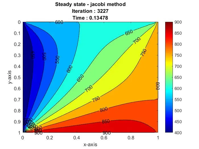
a) Jacobi method:
b) Gauss seidel method:
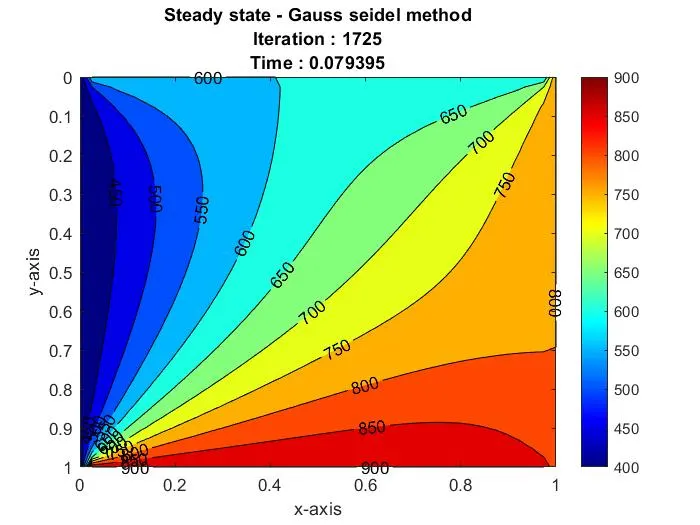
c) SOR method:
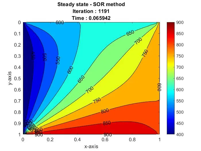
2) Transient-state heat conduction(Explicit):
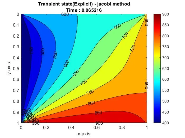
a) Jacobi method:
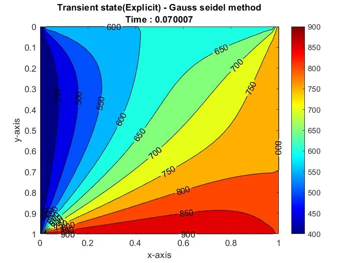
b) Gauss seidel method:
c) SOR method:
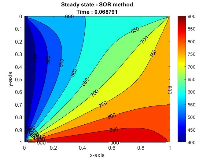
3) Transient-state heat conduction(Implicit):
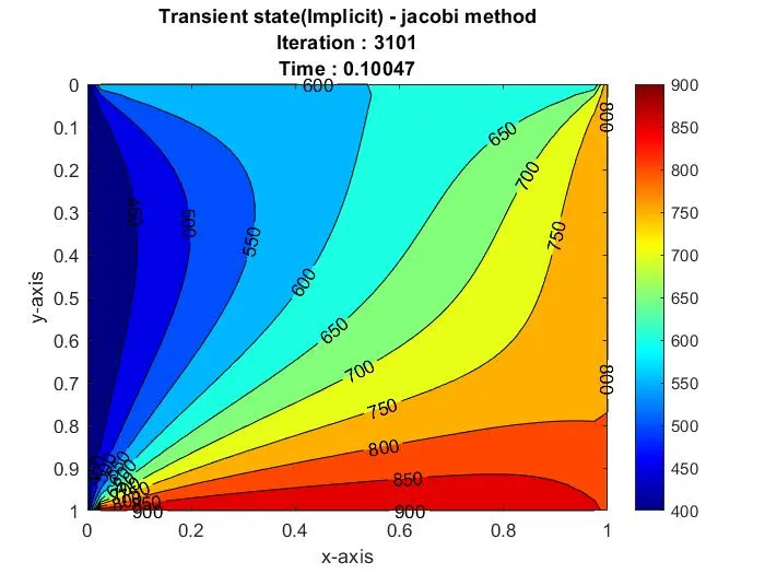
a) Jacobi method:
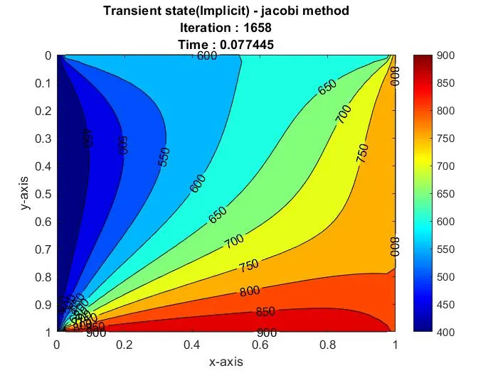
b) Gauss seidel method:
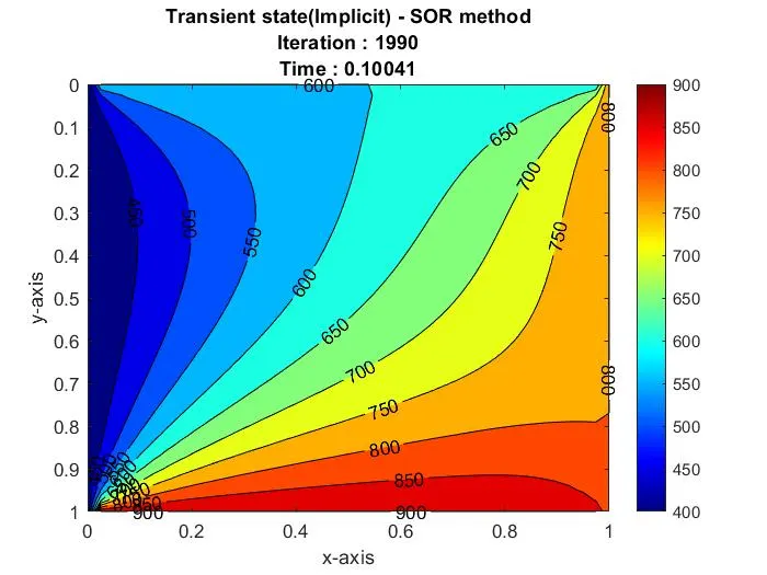
c) SOR method:
Result and discussions:
- From the plots obtained in the steady-state heat conduction simulation, it was found that the successive over relaxation method of iterative solver gives the converged results at minimum number of iterations and time when compared with jacobi and gauss seidel methods.
- In the transient-state heat conduction simulation, the SOR method provides the converged results in minimum time when compared with the other two iterative method.
- Thus, based on the time taken and number of iteration in steady state, Jacobi method > Gauss seidel method > SOR method.
Steady-state vs unsteady analysis:
Based on the number of iterations and time taken by each iterative solver, the time efficient or the fastest iterative method in both steady-state and unsteady analysis was found. The number of iterations on each iterative solver is found.
Steady-state analysis:
| S.No | Iterative solver | Number of iterations | Time taken |
| 1. | Jacobi method | 3227 | 0.13478s |
| 2. | Gauss seidel method | 1725 | 0.079395s |
| 3. | SOR method | 1191 | 0.065942s |
The output plots obtained from all the three iterative solvers are converged. Based on the number of iterations, SOR method gives converged results in minimum number of iterations. It took 1191 iterations where jacobi method took 3227 iterations and gauss seidel method took 1191 number of iterations for the same input values. The SOR method took only 0.065942s to provide the converged results, which is the minimum time when compared with the time taken by the other two methods. Thus, the SOR is the fastest method in a steady state analysis.
Unsteady or Transient analysis:
Explicit:
| S.No | Iterative solvers | Time taken |
| 1. | Jacobi method | 0.065216s |
| 2. | Gauss seidel method | 0.070007s |
| 3. | SOR method | 0.068791s |
The output plots obtained from all the three iterative solvers are converged. In the unsteady state analysis, proper input values should be assigned to get the converged or steady state results. The transient state simulation is a time dependent simulation. So, based on the least time took by the iterative method the fastest metho was found. Based on the time taken by the each iterative solver, the jacobi method took 0.065216s to provide the converged results. The gauss seidel method and the SOR method took 0.070007s and 0.068791s to provide the converged results. Thus, based on the time taken by the method, jacobi method is the fastest iterative method in the unsteady-state or transient analysis under explicit scheme.
Implicit:
| S.No | Iterative solver | Number of iterations | Time taken |
| 1. | Jacobi method | 3101 | 0.10047s |
| 2. | Gauss seidel method | 1658 | 0.077445s |
| 3. | SOR method | 1990 | 0.10041s |
The output plots obtained from all the three iterative solvers are converged. The implicit scheme in the unsteady or transient state analysis depends on the number of iterations and the time taken by the analysis to converged. Based on the number of iterations, gauss seidel method gives converged results in minimum number of iterations. It took 1658 iterations where jacobi method took 3101 iterations and SOR method took 1990 number of iterations for the same input values. The gauss seidel method took only 0.077445s to provide the converged results, which is the minimum time when compared with the time taken by the other two methods. Thus, the gauss seidel method is the fastest method in the unsteady or transient state under implicit condition.
Conclusion:
The successive over relaxation(SOR) iterative method is the best and fastest method beacuse it provides the converged results at less time and low number of iterations when compared it with the jacobi and gauss seidel method in the steady state analysis. In unsteady state analysis, the jacobi method is the fastest method under explicit scheme and the gauss seidel method is the fastest one under implicit scheme. In unsteady state the value of time step play a crucial role to get the converged results.
Stability analysis:
The unstable solution can be analysed by calculating and analysing the approximations made while solving the 2d heat conduction equations. The computational instability is reffered to the consideration of discretization error and round off error occuring while solving the differential equation or the governing equation by different schemes. This error and approximation is occur while solving the governing equation because it changes exponenetially and it have some oscillations. This made the solution that deviate from the exact solution of the governing equation. This phenomenon makes the solution of the governing equation unstable. The iteration solver in solving the solution is made with some assumptions. It too make the solution unstable.
The CFL number or Courant Friedrichs Lewy number play a vital role in obtaining the stable results in the transient state computational analysis. The CFL number can be calculated from the following equation,
`k_1=alpha*((Deltat)/(Deltax^2))`
`k_2=alpha*((Deltat)/(Deltay^2))`
Where `k_1` is the CFL number along x and
`k_2` is the CFL number along y.
The CFL value influence the stability of the solution in the transient condition. In the explicit condition, the CFL number value should be less than 0.5. In the implicit condition, CFL number may have the larger values inorder to get the solution converged. The abnormal CFL value may lead to diffusion in the solution and the solution is blowed up. The following plots exhibit how the solution differes for various CFL values,
Explicit condition:
Initially, the alpha value is set to 1.5 and the CFL value is obtained as 0.4563 for particular dx vand dy value. The plots obtained are shown below,
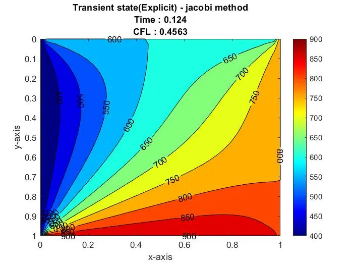
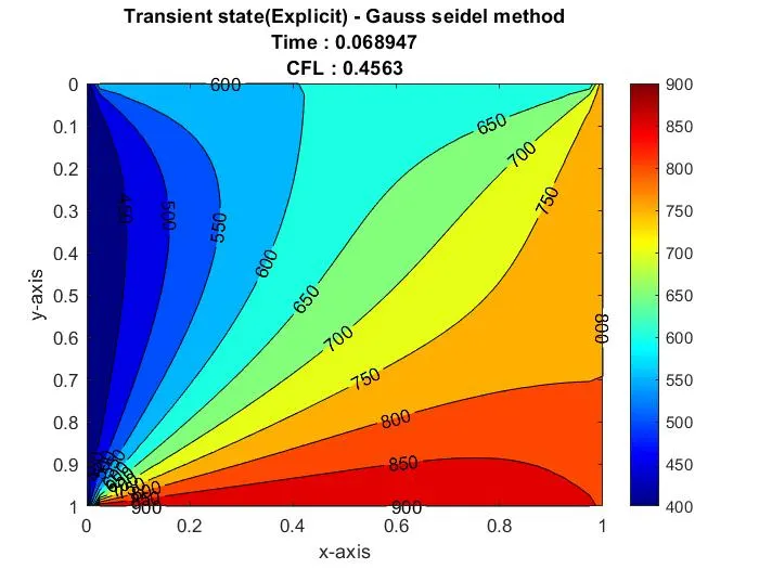
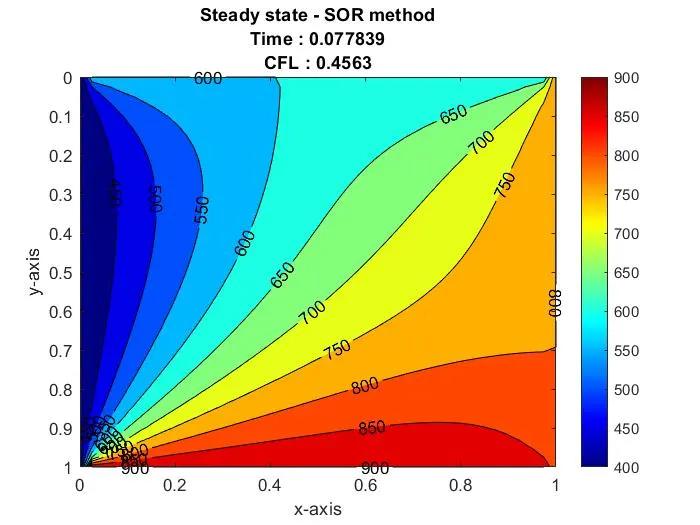
Now the CFL value is increased by increasing the alpha value to 2. Now the CFL value is obtained as 0.6084,
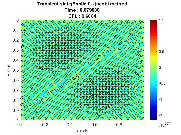
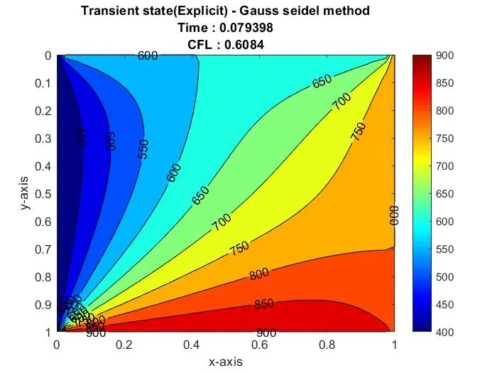
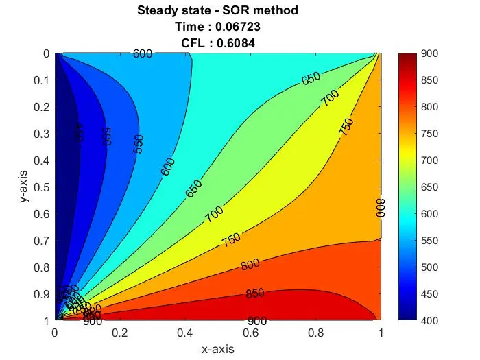
In this condition, the result plot of jacobi method blows up. The gauss seidel and SOR method manage to get the stable or steady state solution for this CFL value.
Now the CFL value is increased by increasing the alpha value to 3. Now the CFL value is obtained as 0.9126,
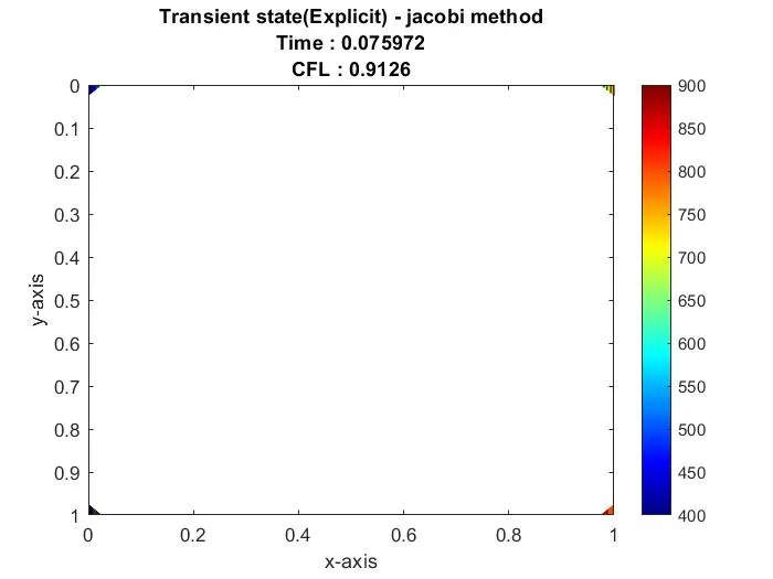
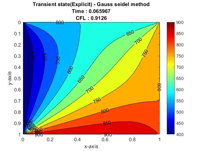
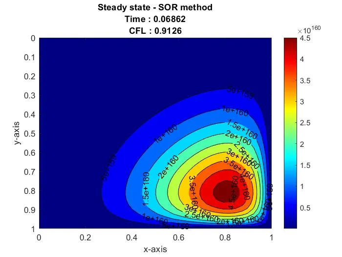
In this condition, the jacobi method blows up completely and SOR method gives an unstable blowed solution. But still gauss seidel method manages to provide the optimum or steady plot.
Now the CFL value is increased by increasing the alpha value to 4. Now the CFL value is obtained as 1.2168,
In this condition, the three iterative solvers blowed completely and didn't show the plot. Thus, when the CFL value goes beyond 1, the three iterative solvers blow up completely and become unstable. It clearly explains the influence of CFL number in the stability of the problem.
Implicit condition:
In the implicit condition, the CFL value didnot affect the stability of the solution considerably. By changing the CFL value to the abnormal value may made the solution to unstable.
Thus, the CFL number defines the stability of the solution in the transient condition especially under explicit scheme.
References:
- COMPUTATIONAL FLUID DYNAMICS - The Basics with Applications by John D. Anderson, Jr.
- https://en.wikipedia.org/wiki/Heat_equation
- https://en.wikipedia.org/wiki/Thermal_conduction
- https://in.mathworks.com/help/matlab/ref/contourf.html
- https://in.mathworks.com/help/matlab/ref/jet.html
Keywords:
CFD, MATLAB, Discretization, Iterative solvers, Jacobi method, Gauss seidel method, SOR method, steady-state, transient-state.