Simulation of fluid flow thermal mixing in the T-junction using k-epsilon and k-omega SST models for different momentum ratios in ANSYS Fluent
PROBLEM SPECIFICATION:
For this project, we have created two versions of the T-junction. One of them is longer than the other.
Our job is to set up steady-state simulations to compare the mixing effectiveness when the hot inlet temperature is 360C & the Cold inlet is at 190C.
Use the k-epsilon and k-omega SST model for the first case and based on the judgment, we’ll use the more suitable model for further cases. Giving the reason for choosing a suitable model is compulsory.
- Case 1
- Short T-junction with a hot inlet velocity of 3m/s.
- Momentum ratio of 2, 4.
- Case 2
- Long T-junction with a hot inlet velocity of 3m/s.
- Momentum ratio of 2, 4.
Momentum ratio = velocity at cold inlet / velocity at hot inlet
In a table, compare the following values from the 2 cases.
- Cell count
- Average outlet temperature
- Number of iterations for convergence
Expected results:
- Velocity and temperature contour plots on the cut planes along and across the pipe.
- Velocity and temperature line plots along and across the length of the pipe.
- Perform Mesh independent study for any one case.
- Discuss the effect of length and momentum ratio on results.
For each simulation, we need to show the convergence plot.
INTRODUCTION:
In this project, we’re going to simulate the fluid flow mixing in T-junction using different turbulence models for different momentum ratio. We will set up the steady-state simulations to compare the thermal mixing effectiveness when the hot inlet temperature is 360C & the cold inlet is at 190C. The turbulence models we’re going to use for our first case are k-epsilon and k-omega SST, and based on the results we’ll further use any of them accordingly for our second case. Here we are simulating for two different geometries of T-junction; one is longer than the other. The motive behind choosing two different geometries is to get a better understanding of mixing effectiveness. We compute the standard deviation of temperature at the outlet to quantify the degree of mixing. We also compute the velocity and temperature fields to show the quality of mixing we’re getting in different setups. After analyzing the results got from both the models and comparing them with the analytical solution; we will decide which turbulence model is best suited for this simulation.
THEORY:
Junctions between pipes can involve the mixing or splitting of fluids. In single-phase flow, the flows about the junction are very complex with recirculation possible in the outlet pipe(s), features first observed by Leonardo da Vinci.
The T-junction is used for the division or the combination of fluid flow, and it is a very important part of the pipe-line system. It can vary in shape, and we primarily use it for dividing or combining of flow in a pipeline. However, the T-junction can be also used for the mixing of two different liquids, liquid, and gas, or two different gasses. T-junctions are present in a wide range of industries and facilitate the mixing of fluids that are often at different temperatures. In industrial process engineering, mixing is a unit operation that involves the manipulation of a heterogeneous physical system intending to make it more homogeneous. We perform mixing to allow heat and/or mass transfer to occur between one or more streams, components, or phases. Modern industrial processing almost always involves some form of mixing. The T-junction is a mixing mechanism, and it utilizes a specifically engineered internal geometry to efficiently mix two fluid streams into one combined stream. T-junctions are widely used in the petrochemical, HVAC industry, etc. in which two fluid streams with different physical and/or chemical properties mix together.
ANALYTICAL SOLUTION:
Preliminary Data:-
Fluid: Air
Density: `ρ_(air)=1.225 (kg)/m^3`
Specific Heat: `C_p=1006.43 J/(Kg.K)`
Area (hot inlet): `A_(hot)=0.0009 m^2`
Area (cold inlet): `A_(cold)=0.0002 m^2`
Temperature (hot inlet): `T_(hot)=36^0 C`
Temperature (cold inlet): `T_(cold)=19^0 C`
When momentum ratio=2: Velocity @hot inlet, `V_(hot)=3 m/s` and Velocity @cold inlet, `V_(cold)=6m/s`
When momentum ratio=4: Velocity @hot inlet, `V_(hot)=3 m/s` and Velocity @cold inlet, `V_(cold)=12m/s`
Reference formula for temperature: `T_(mix)=(m_(hot)*T_(hot)+m_(cold)*T_(cold))/(m_(hot)+m_(cold))`
Where, mass flow rate of hot fluid, `m_(hot)=ρ_(air)*A_(hot)*V_(hot)`
mass flow rate of cold fluid, `m_(cold)=ρ_(air)*A_(cold)*V_(cold)`
`T_(hot)=` Temperature of hot fluid
`T_(cold)=` Temperature of cold fluid
a) When momentum ratio=2:
`T_(mix)=[((ρ_(air)*A_(hot)*V_(hot) )*T_(hot)+(ρ_(air)*A_(cold)*V_(cold ))*T_(cold))/((ρ_(air)*A_(hot)*V_(hot ))+(ρ_(air)*A_(cold)*V_(cold) ) )]`
`T_(mix)=[((1.225*0.0009*3)*36+(1.225*0.0002*6)*19)/((1.225*0.0009*3)+(1.225*0.0002*6) )]`
`T_(mix)=30.769^0C`
b) When momentum ratio=4:
`T_(mix)=[((ρ_(air)*A_(hot)*V_(hot) )*T_(hot)+(ρ_(air)*A_(cold)*V_(cold ))*T_(cold))/((ρ_(air)*A_(hot)*V_(hot ))+(ρ_(air)*A_(cold)*V_(cold) ) )]`
`T_(mix)=[((1.225*0.0009*3)*36+(1.225*0.0002*12)*19)/((1.225*0.0009*3)+(1.225*0.0002*12) )]`
`T_(mix)=28^0C`
Case 1: Short T-junction with a hot inlet velocity of 3m/s and with momentum ratio of 2 & 4
PRE-PROCESSING AND SIMULATION SETUP:
Geometry:
We have created geometry in SolidWorks and then saved in ‘.STEP’ file to import in ANSYS SpaceClaim for the CAD cleanup process. The Short T-junction geometry with dimensions has been shown below and remember that the images shown below are from SolidWorks, and this is not the final geometry we are going to use for simulation.
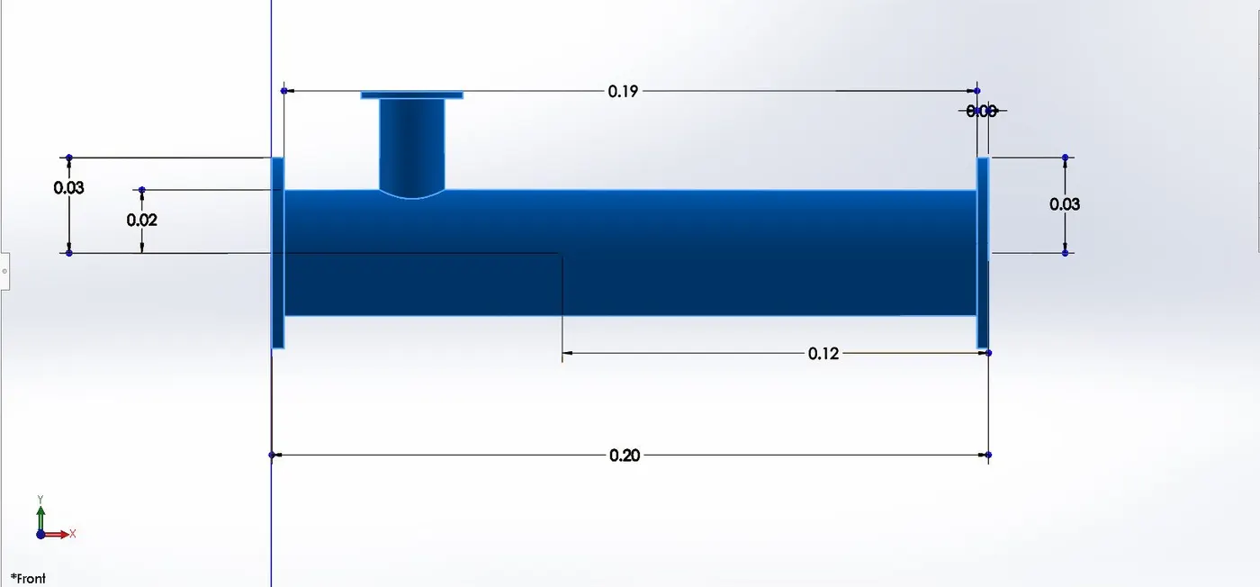
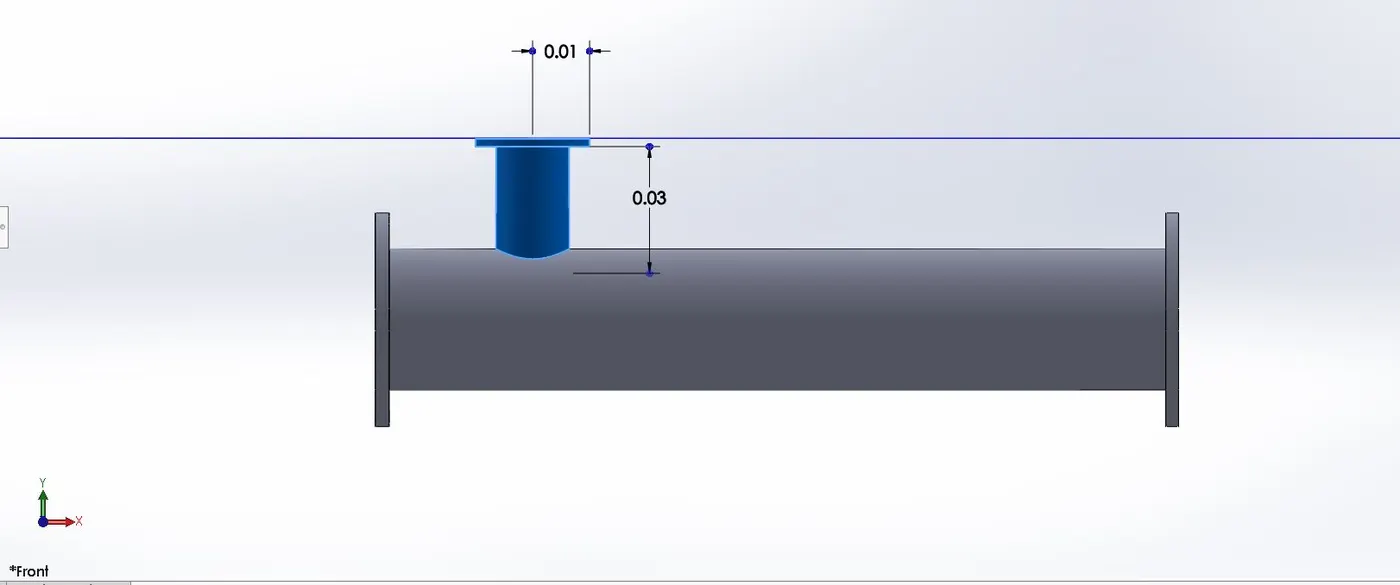
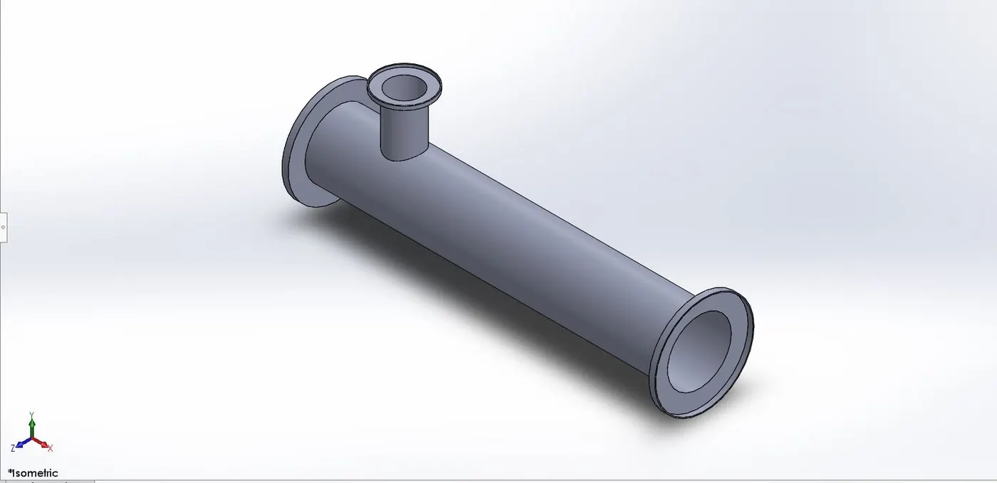
After creating the geometry in SolidWorks, we’ll import the geometry in ANSYS SpaceClaim for the CAD cleaning process. Here in the CAD cleaning process we’ll extract the flow volume field from the model and the extracted volume is shown below:
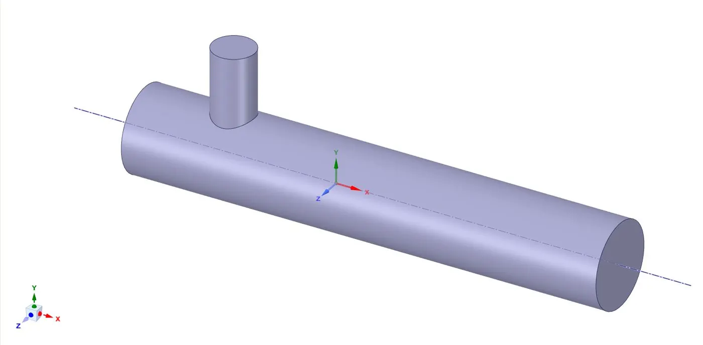
The above geometry is the final short T-junction geometry that we’re going to use in our first case simulation. Hiding the geometry will not affect the object’s inclusion in the simulation. To avoid the hidden geometry to be involved in the simulation, use suppress physics option for the solid geometry.
Meshing:
We use ANSYS inbuilt Meshing tool for the discretization of our flow domain for solving. Since here we are also going to perform the ‘Grid Dependency Test’ to ensure that the results are obtained are independent of the mesh size. Therefore, a coarse mesh (default settings; element size=5e-003m), medium mesh (element size=3.5e-003m), and fine mesh (element size=2e-003m) are generated accordingly. But for later simulations, we’ll use fine mesh only for better; near the wall predictions.
Coarse Mesh: default settings; element size=5e-003m
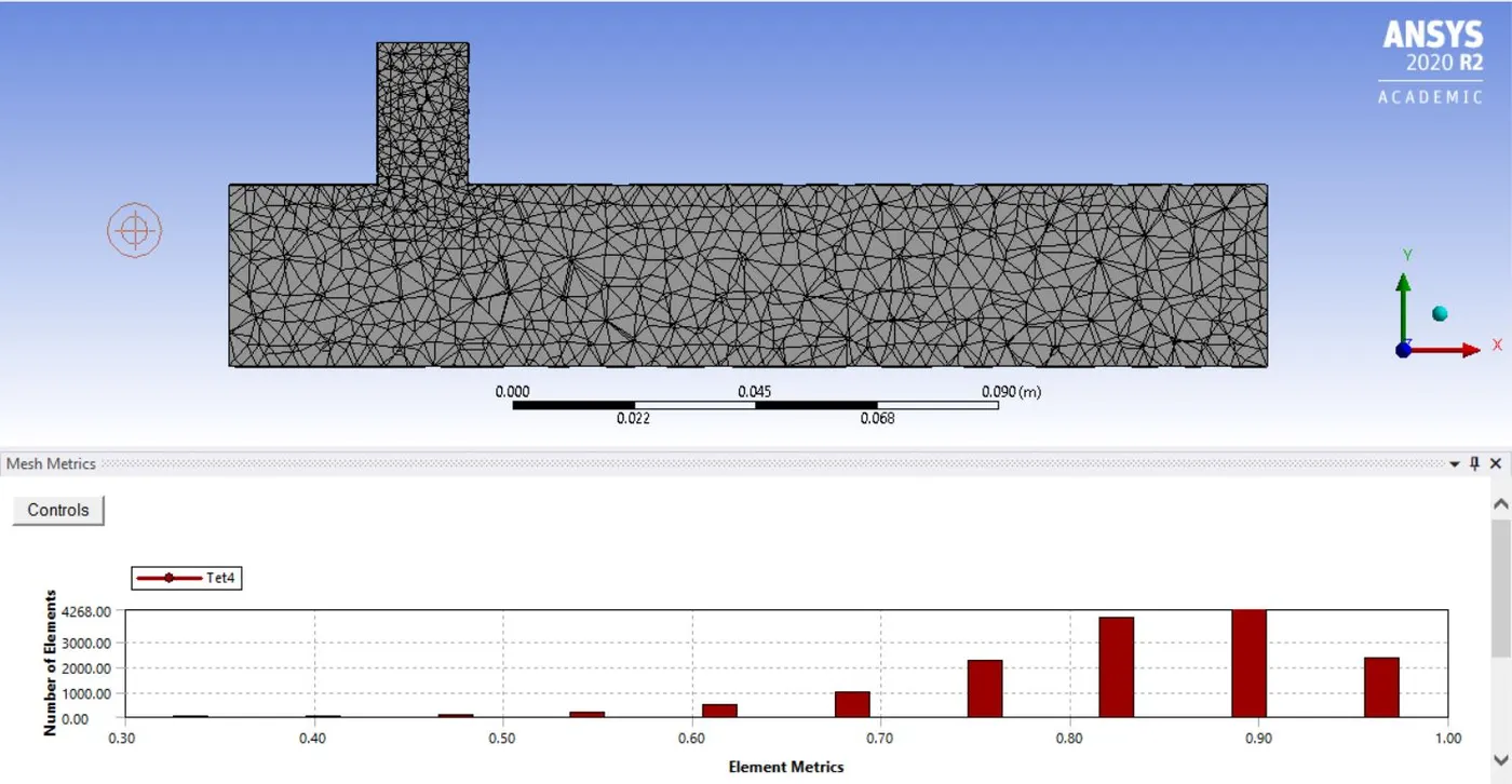
Medium Mesh: element size=3.5e-003m
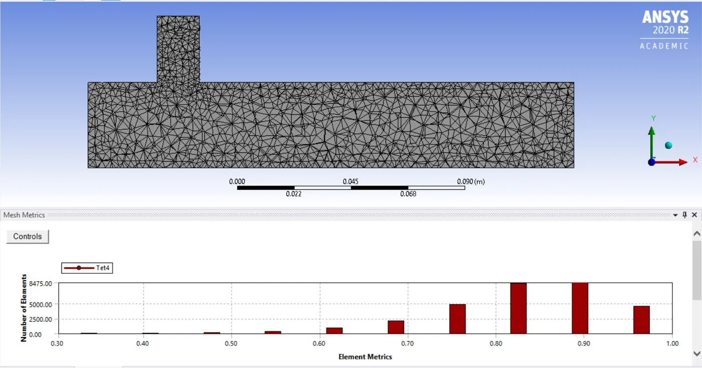
Fine Mesh: element size=2e-003m
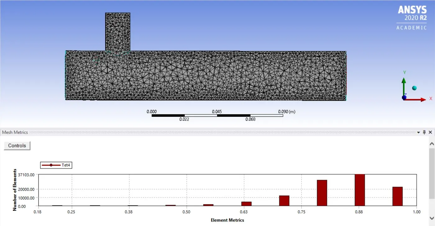
Solver Settings:
ANSYS Fluent is used to set up the flow conditions. Here we apply different boundary conditions, like for inlet, outlet, and wall boundary conditions. For initialization, we’ll use ‘Hybrid initialization’. In our grid independence test, we’ll use the ‘k-epsilon realizable’ turbulence model and for further simulations, we’ll use both the models accordingly for momentum ratio= 2 and 4.
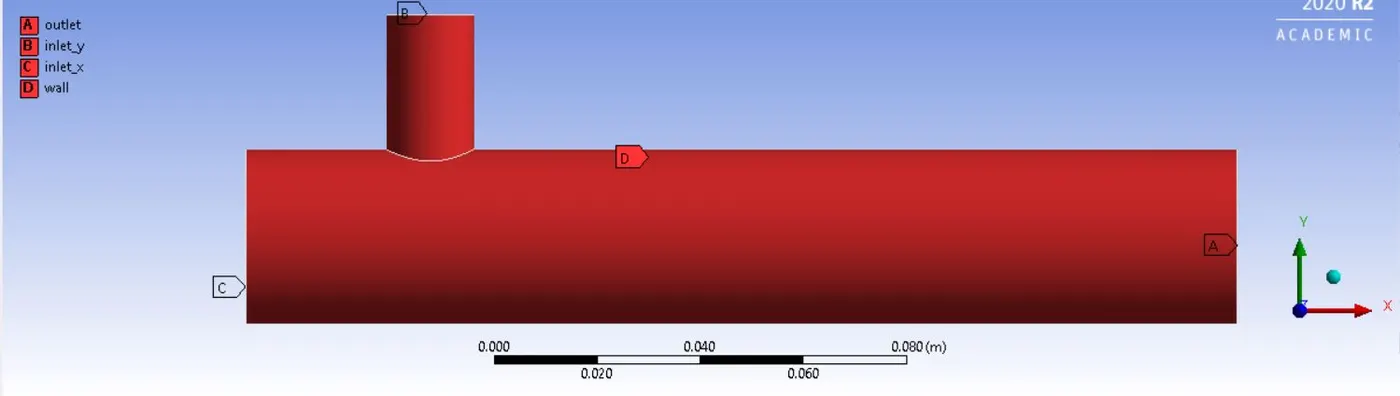
Boundary conditions for inlet, outlet, and wall are:
a) For momentum ratio=2:
inlet_x (hot air inlet): velocity=3m/s; temperature=`36^0C`
inlet_y (cold air inlet): velocity=6m/s; temperature=`19^0C`
outlet: pressure=0 Pa
wall: no-slip condition
b) For momentum ratio=4:
inlet_x (hot air inlet): velocity=3m/s; temperature=`36^0C`
inlet_y (cold air inlet): velocity=12m/s; temperature=`19^0C`
outlet: pressure=0 Pa
wall: no-slip condition
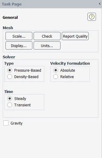
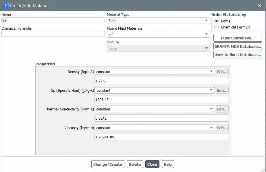
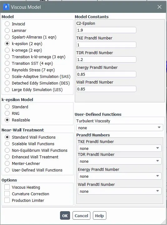
For our first case, we’ll use k-epsilon realizable model and k-omega SST model one by one to get a better understanding of both the models. Snippets for different solver settings are shown below:
k-epsilon turbulence model settings:
k-omega SST model settings:
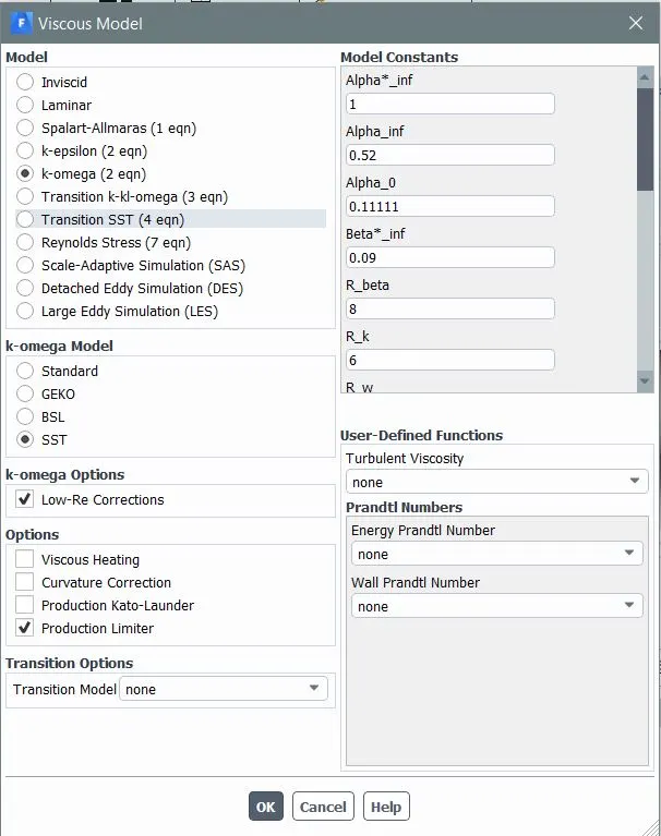
NOTE: The above solver settings will be the same for further simulations as well. Don’t forget to check the energy option in the physical settings box before proceeding for hybrid initialization. Also, the number of iterations completely depends on the convergence of the solution, and here we are taking a different numbers of iterations for different simulations. We’ll run a particular simulation until we reach a converged solution and remember that the runtime will differ from simulation to simulation.
POST-PROCESSING:
Grid Dependency Test Results: (using a k-epsilon model with momentum ratio of 2)

From the above results, we are totally satisfied and can say that the results are grid independence. The errors (w.r.t. analytical solution results) are in tolerable range and we can move further in the post-processing step.
Results and Discussions for Case 1:
a) Momentum ratio=2:
Residual plot:
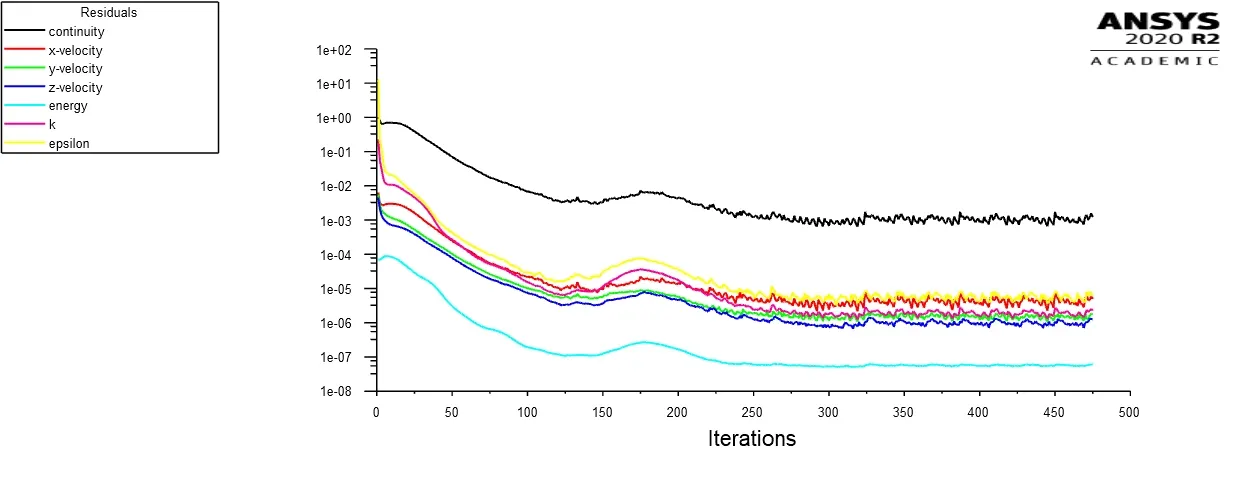
k-epsilon model:
k-omega SST model:
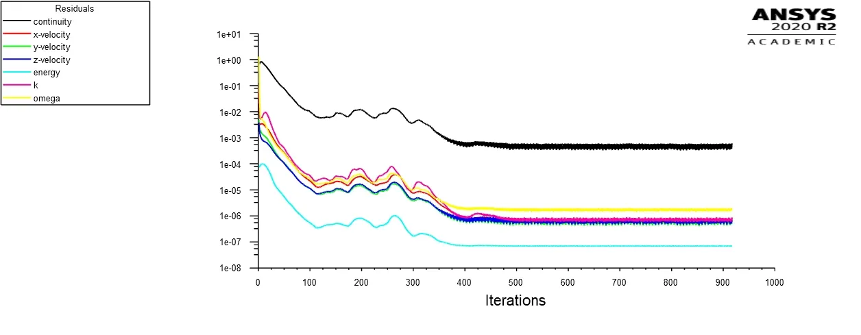
From the above plot of residuals, we can observe that the solution for the k-epsilon model converges near 250 iterations, whereas the k-omega SST model converges near 450 iterations.
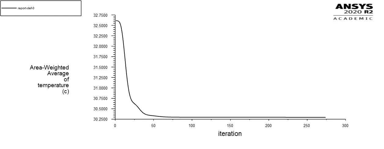
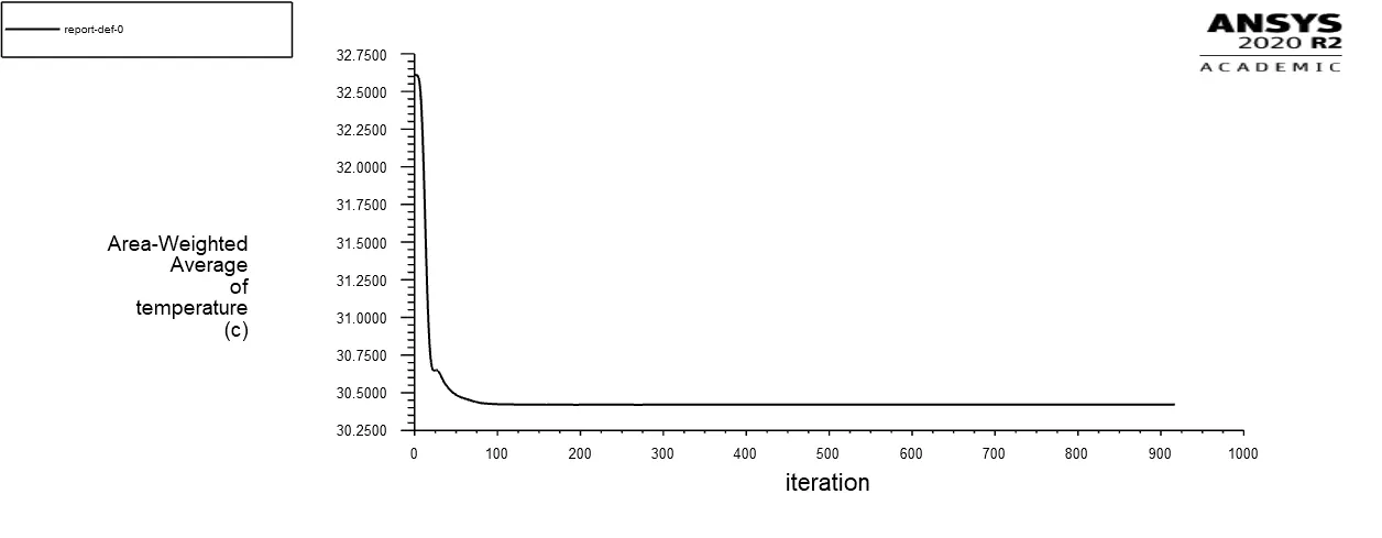
Plot for Area-Weighted Average of temperature at the outlet:
k-epsilon model:
k-omega SST model:
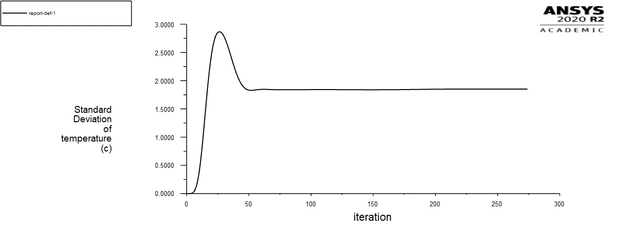
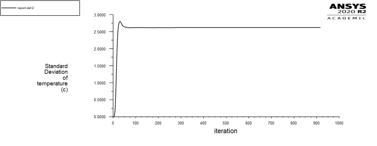
Plot for Standard Deviation of temperature at the outlet:
k-epsilon model:
k-omega SST model:
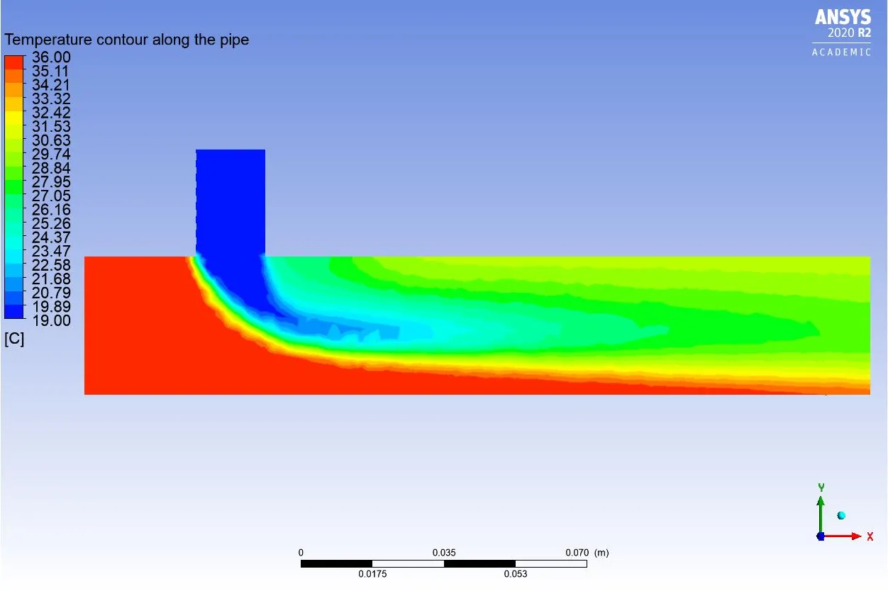
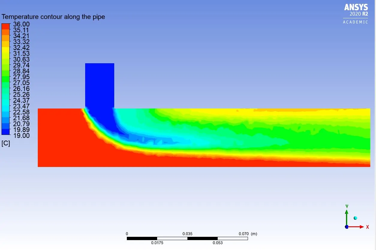
Temperature contour along the pipe:
k-epsilon model:
k-omega SST model:
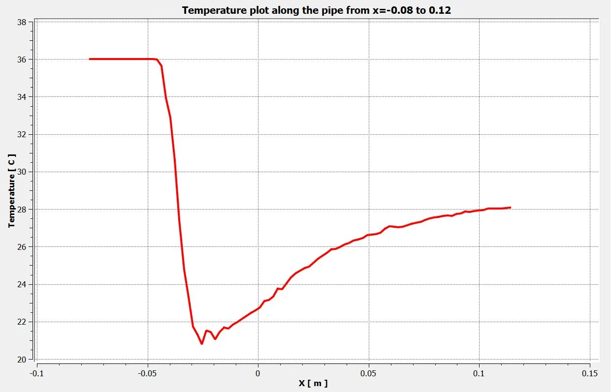
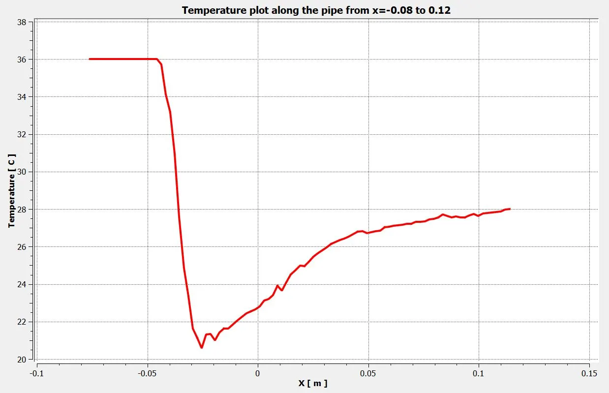
Temperature plot along the pipe from x=-0.08 to x=0.12:
k-epsilon model:
k-omega SST model:
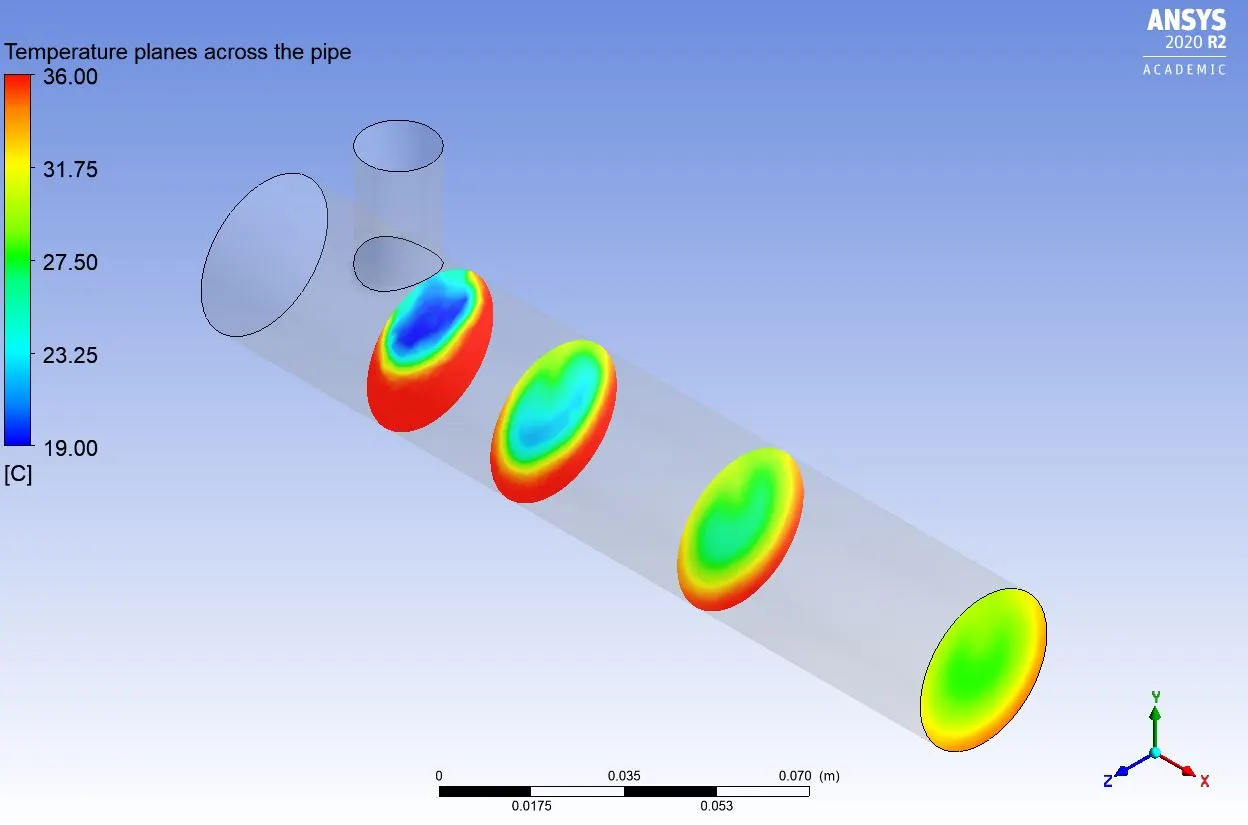
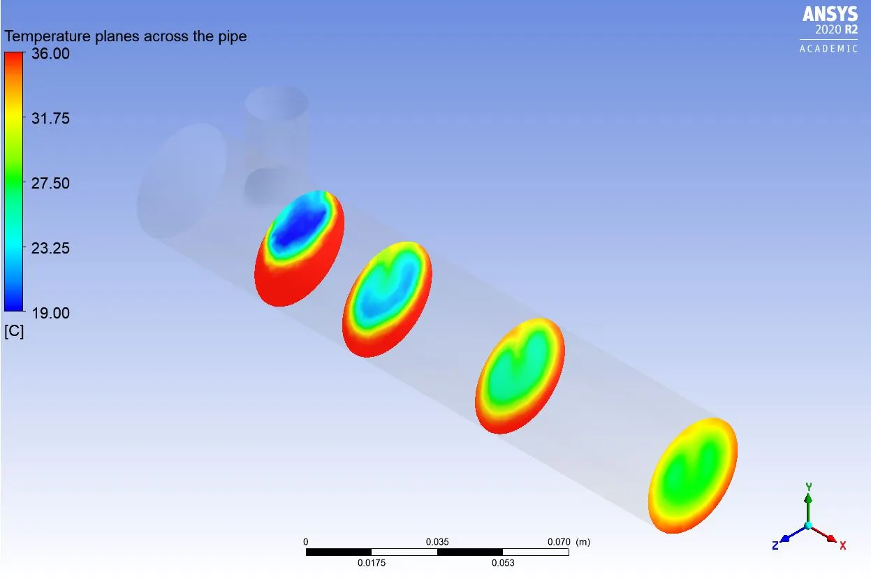
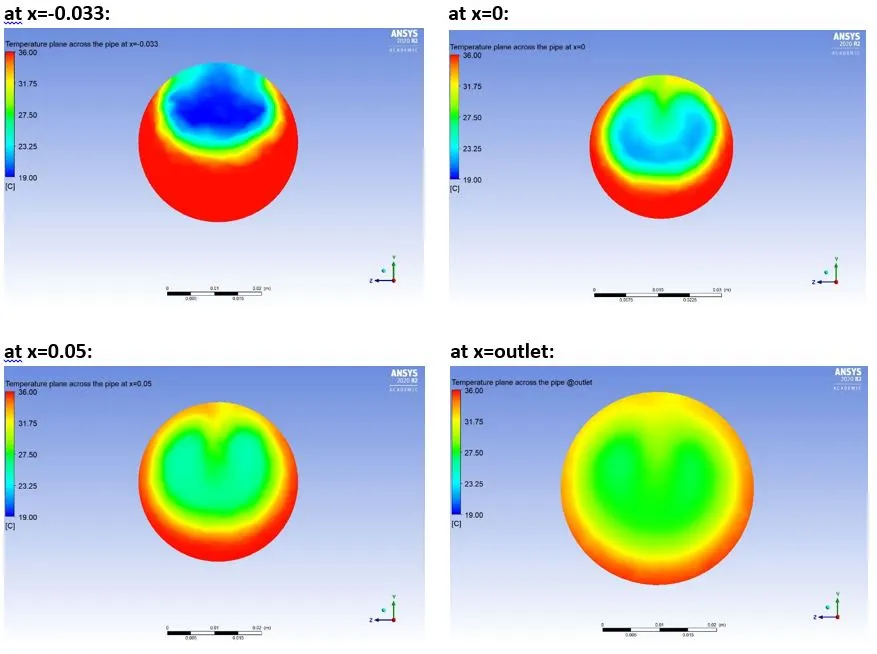
Temperature planes at different distances across the pipe:
k-epsilon model:
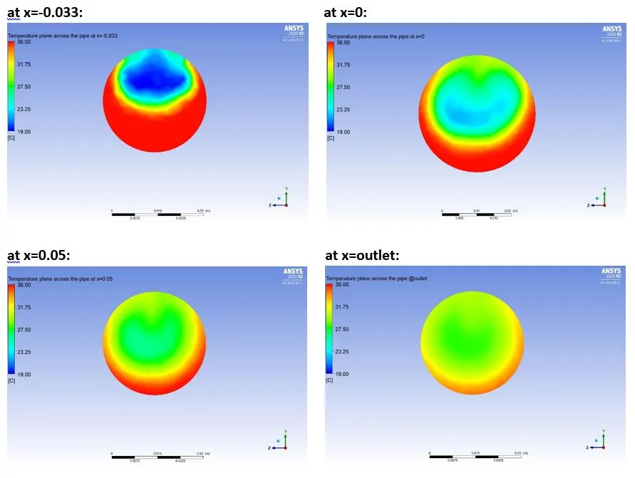
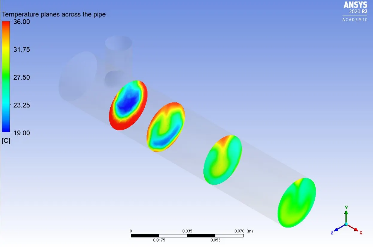
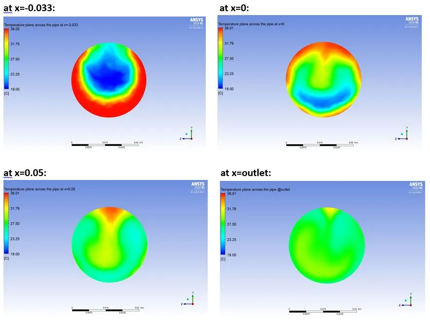
k-omega SST model:
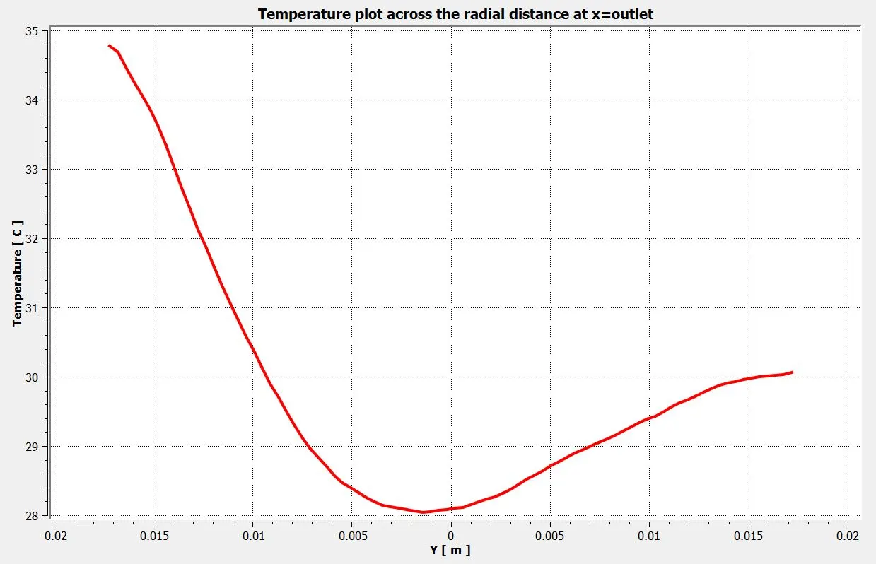
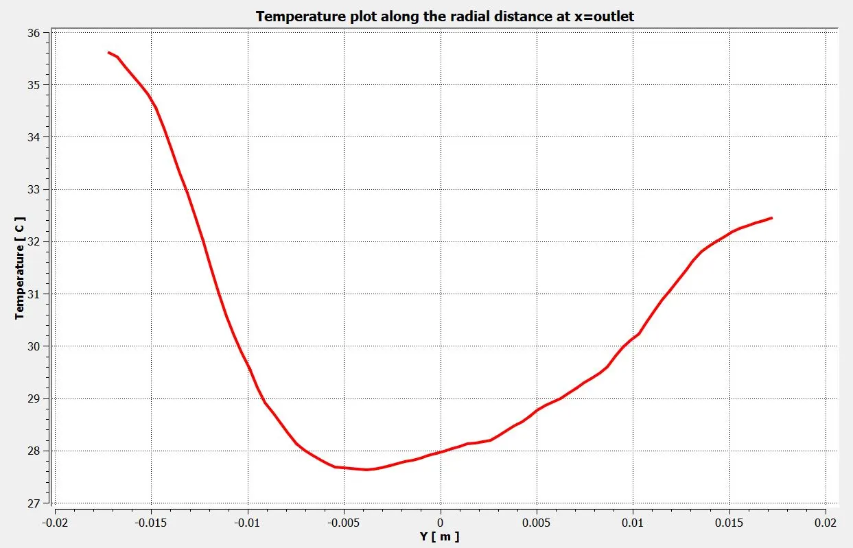
Temperature plot along the radial distance at the outlet:
k-epsilon model:
k-omega SST model:
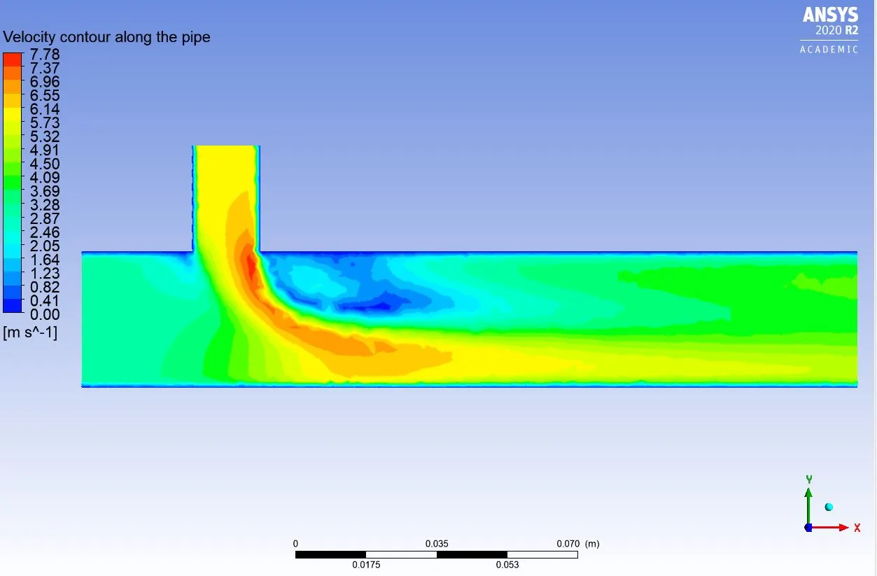
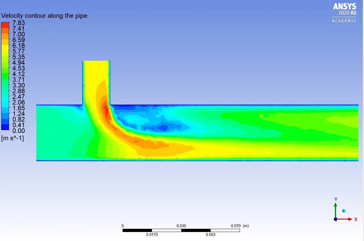
Velocity contour along the pipe:
k-epsilon model:
k-omega SST model:
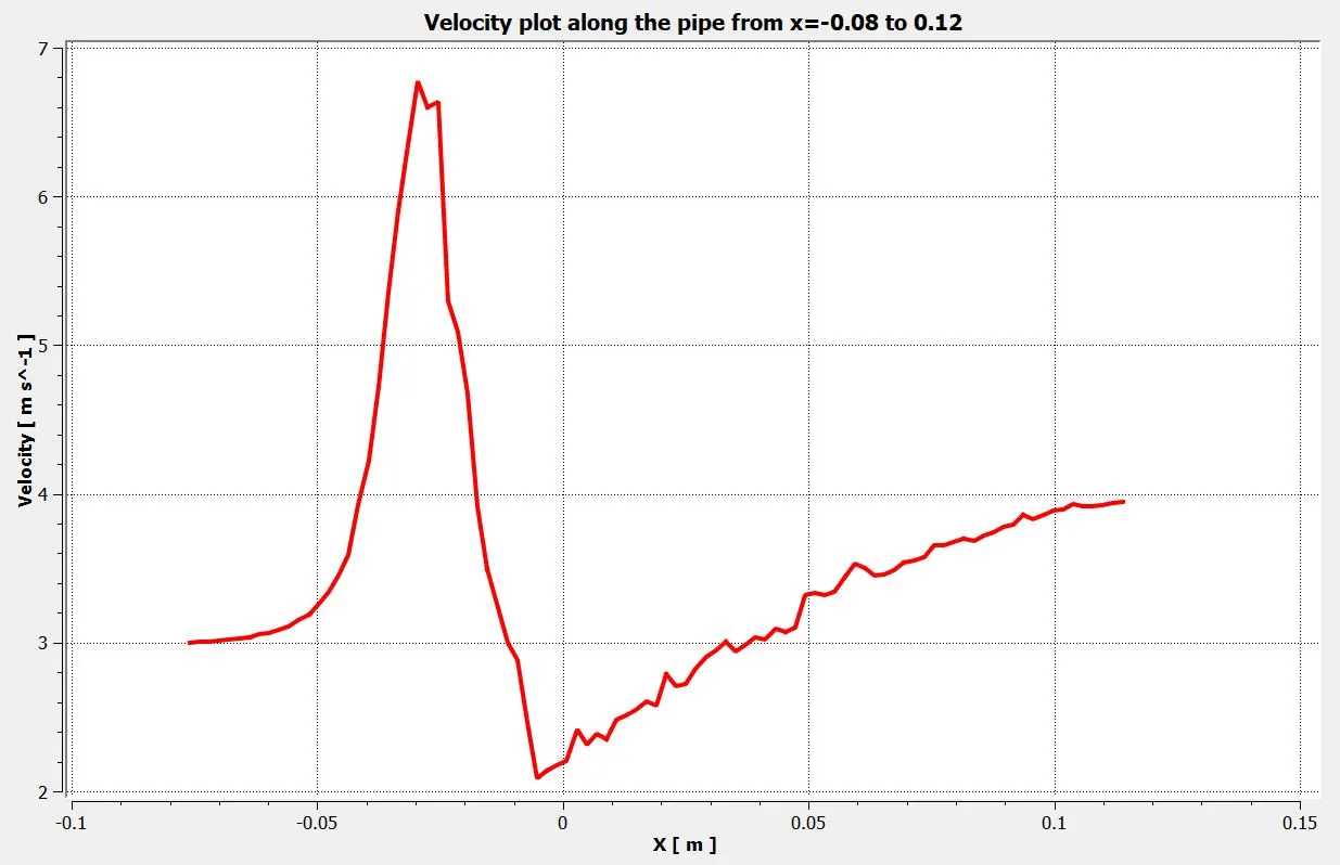
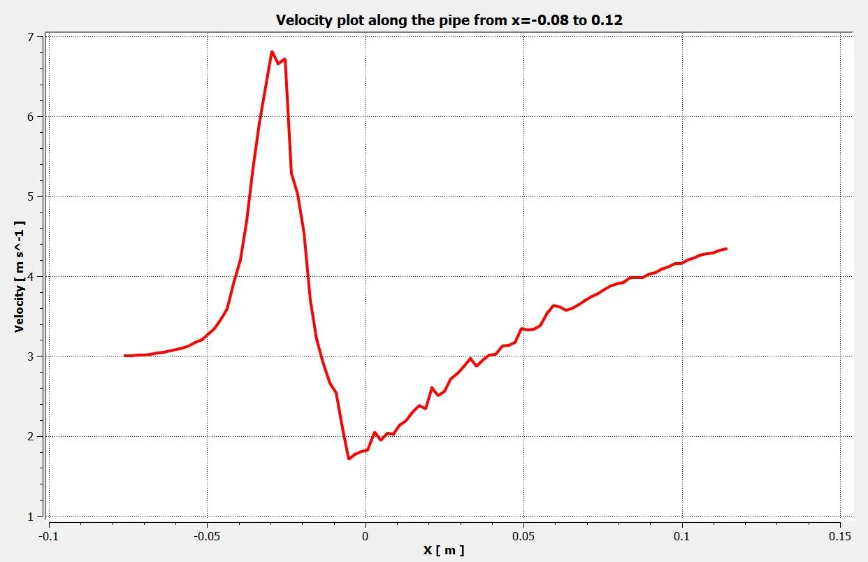
Velocity plot along the pipe from x=-0.08 to x=0.12:
k-epsilon model:
k-omega SST model:
Velocity planes at different distances across the pipe:
k-epsilon model:
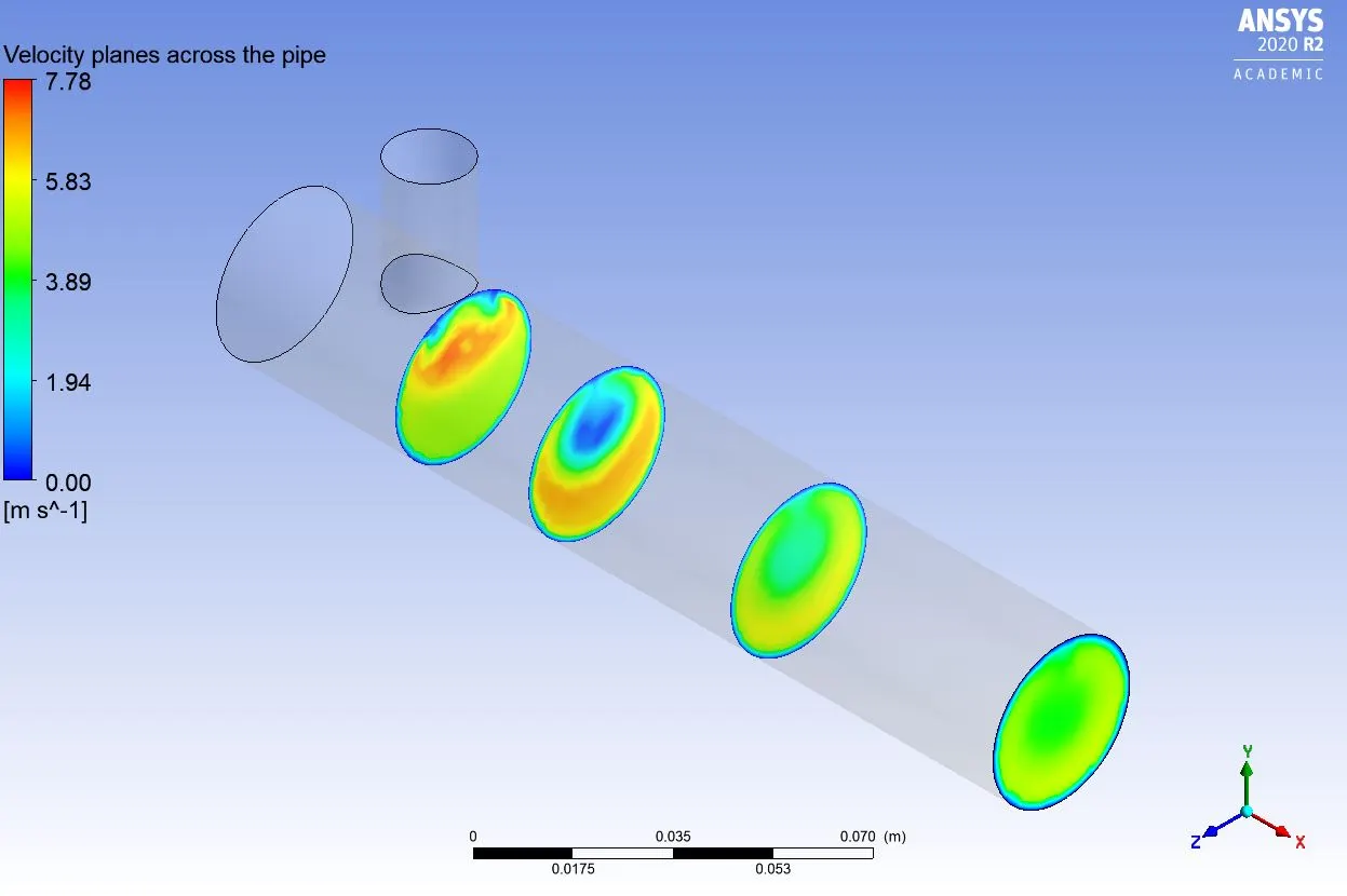
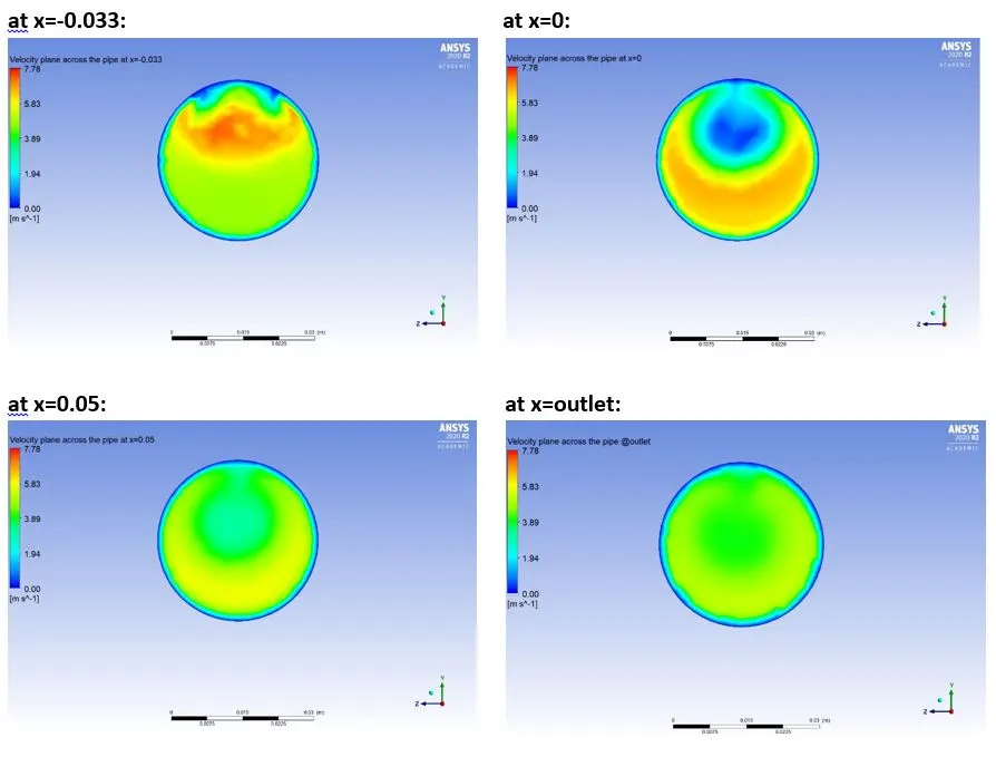
k-omega SST model:
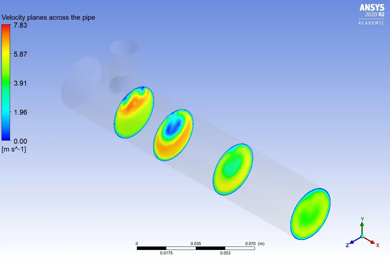
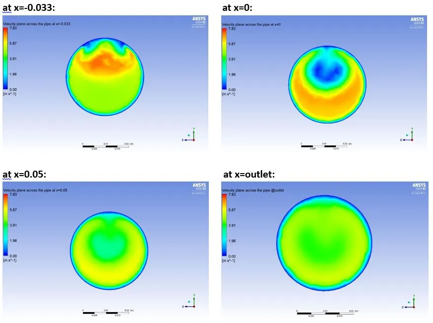
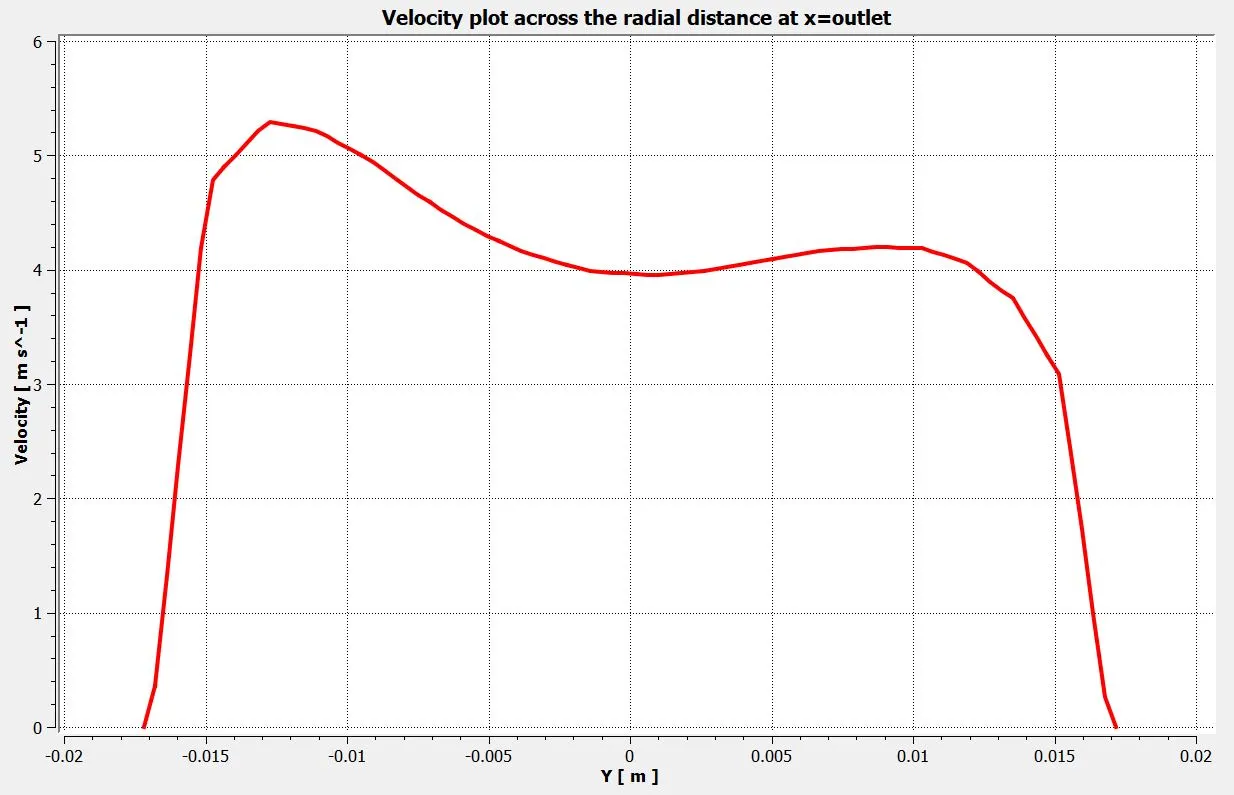
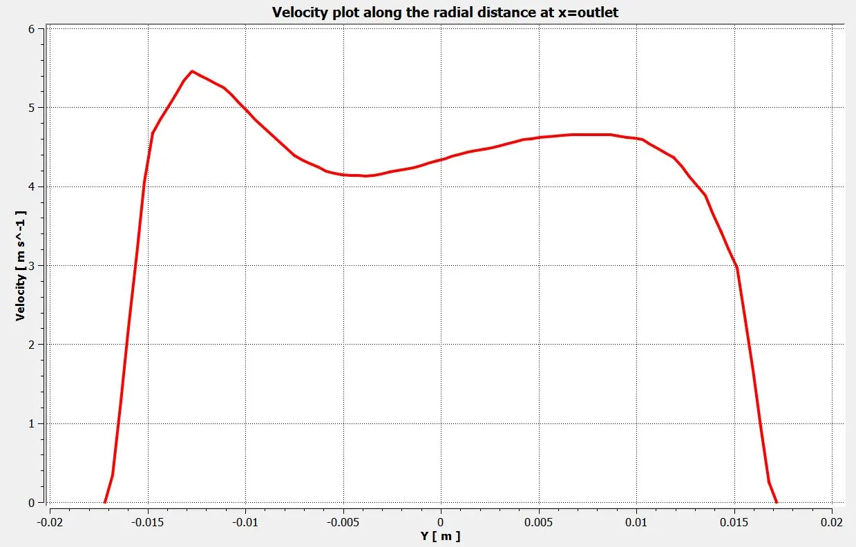
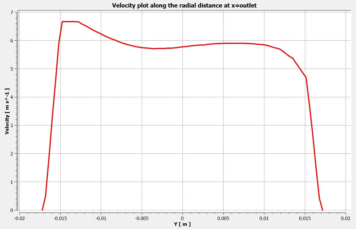
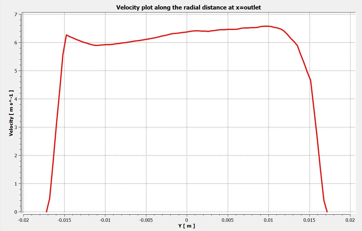
Velocity plot along the radial distance at the outlet:
k-epsilon model:
k-omega SST model:
b) Momentum ratio=4:
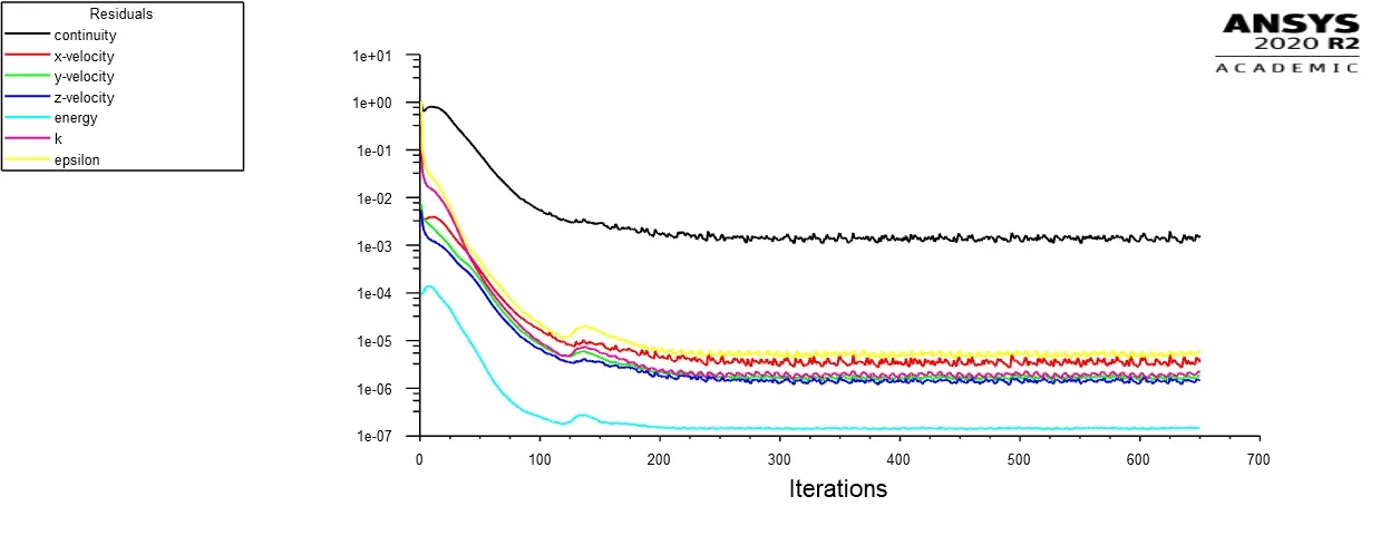
Residual plot:
k-epsilon model:
k-omega SST model:
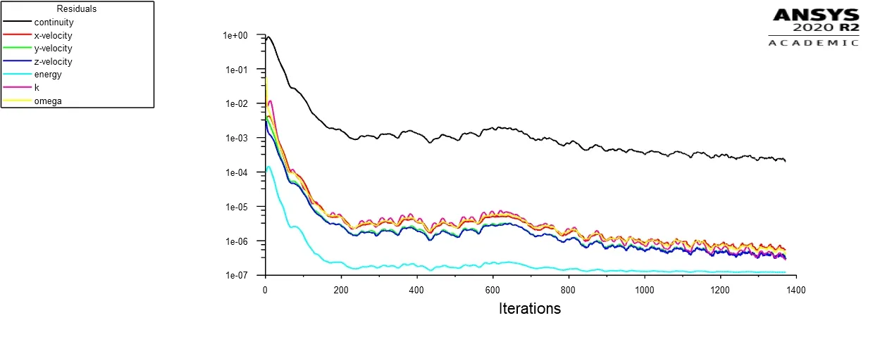
From the above plots of residuals, we can observe that the solution for the k-epsilon model converges near 200 iterations, whereas the k-omega SST model converges near 800 iterations.
Plot for Area-Weighted Average of temperature at the outlet:
k-epsilon model:
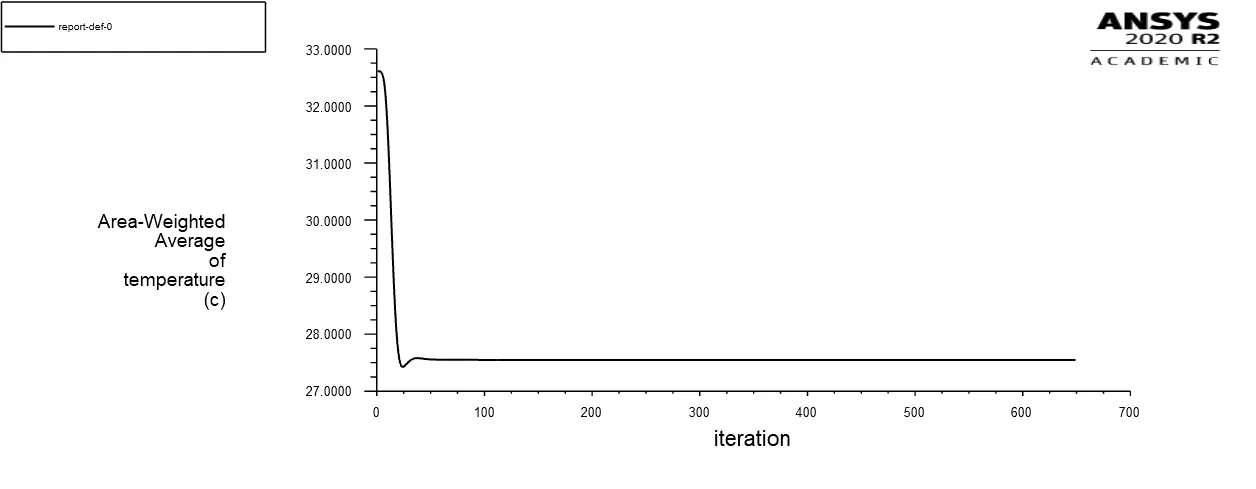
k-omega SST model:
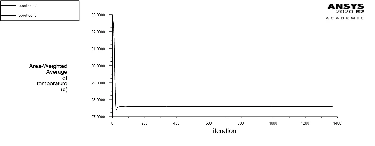
Plot for Standard Deviation of temperature at the outlet:
k-epsilon model:
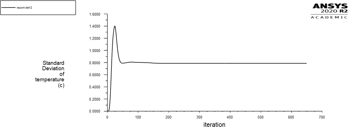
k-omega SST model:
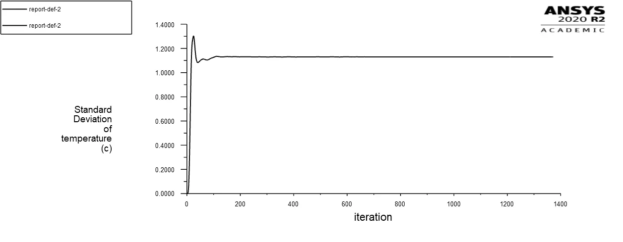
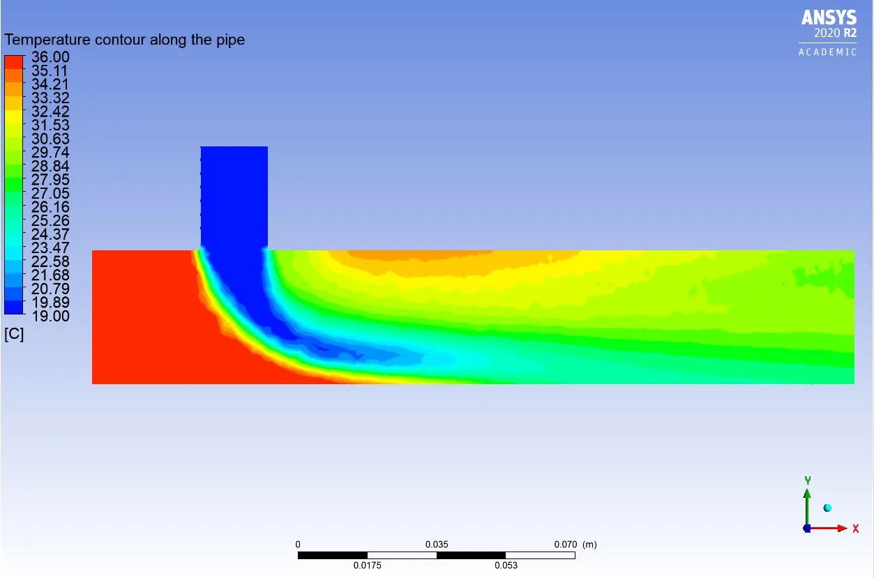
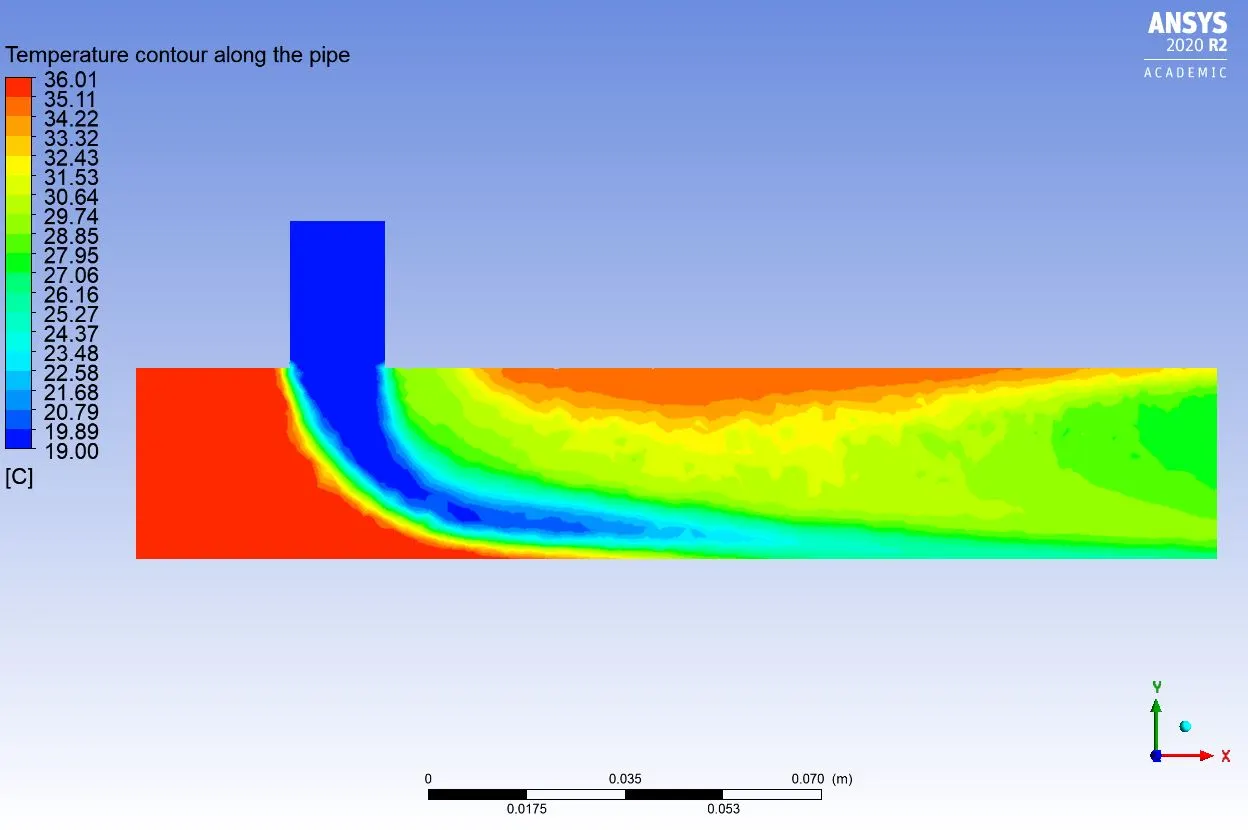
Temperature contour along the pipe:
k-epsilon model:
k-omega SST model:
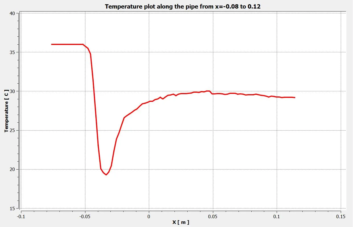
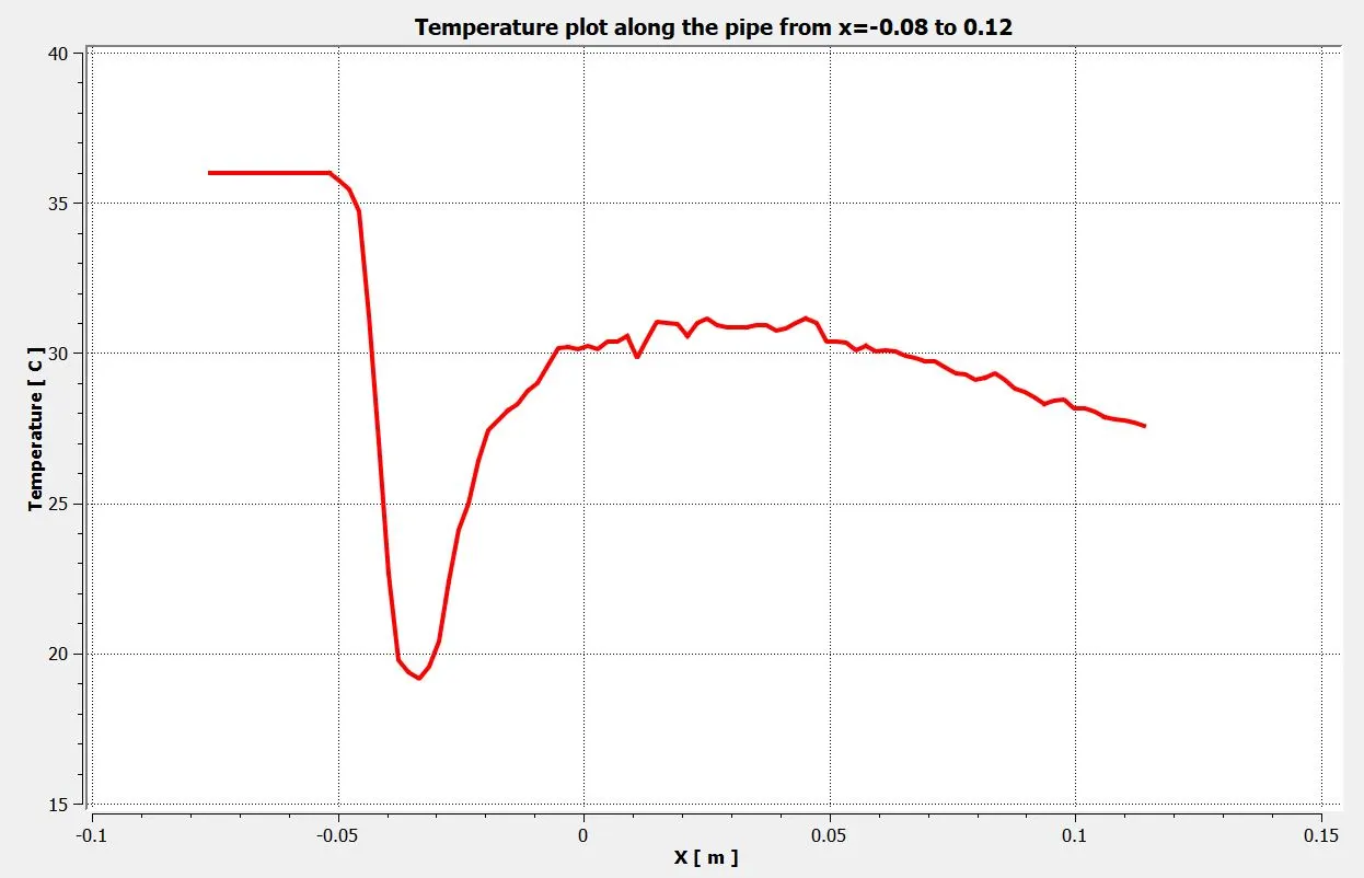
Temperature plot along the pipe from x=-0.08 to x=0.12:
k-epsilon model:
k-omega SST model:
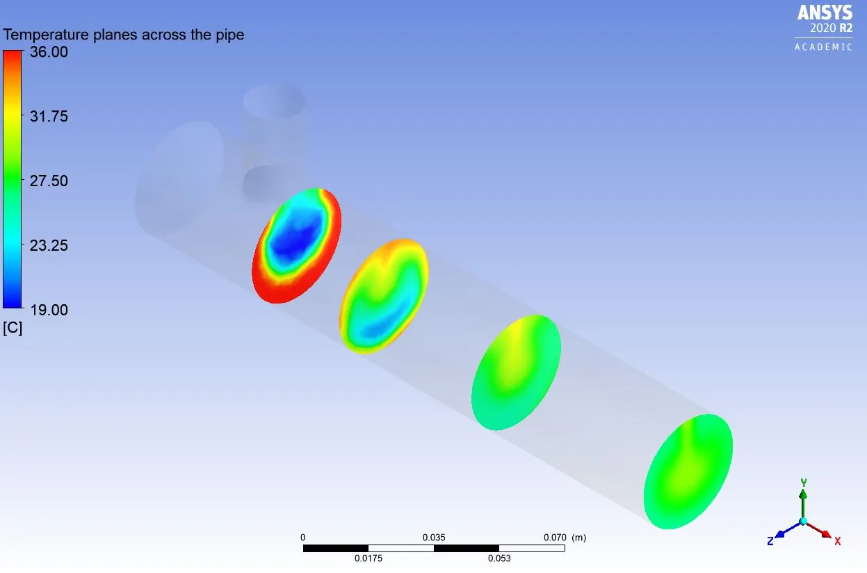
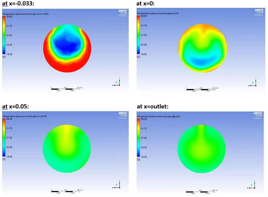
Temperature planes at different distances across the pipe:
k-epsilon model:
k-omega SST model:
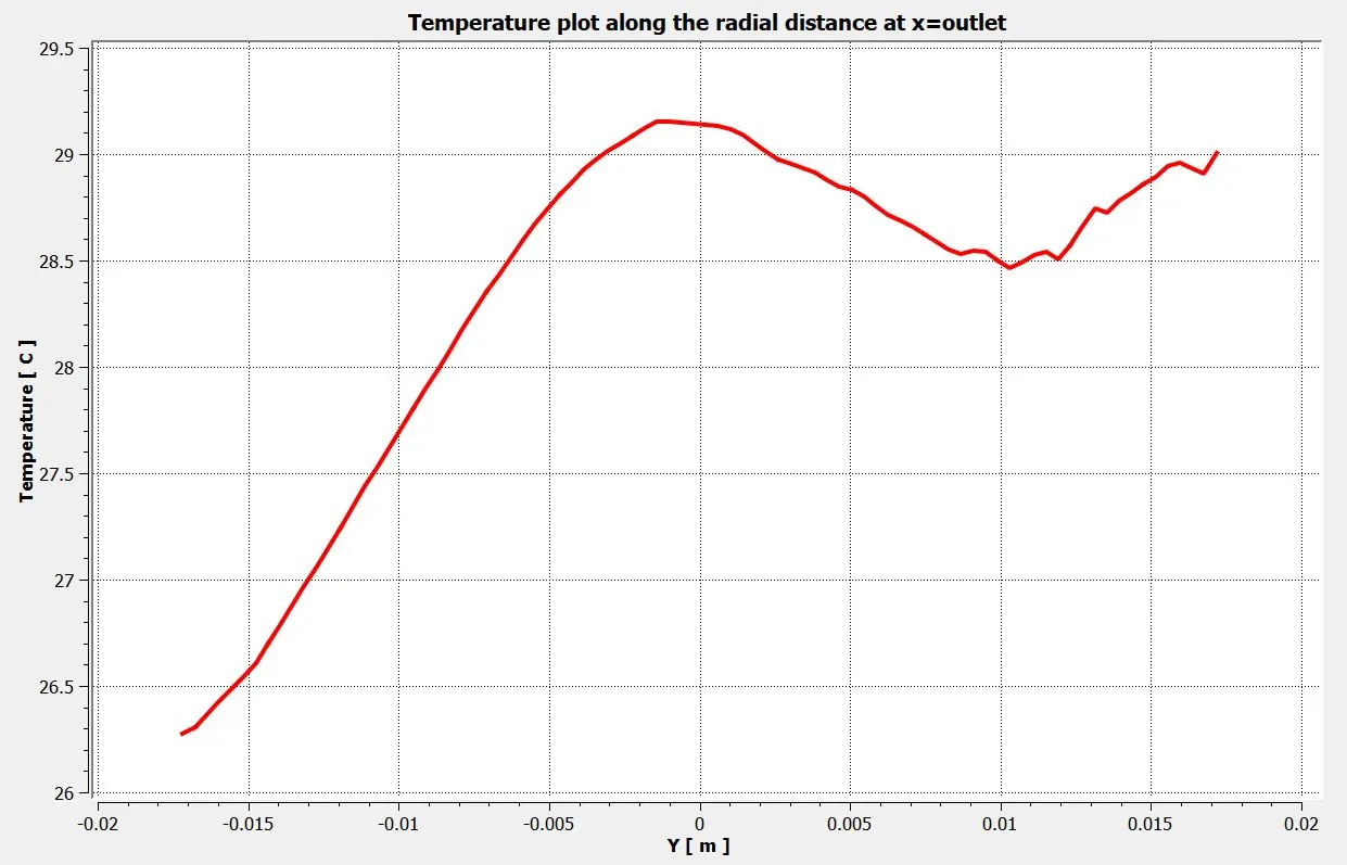
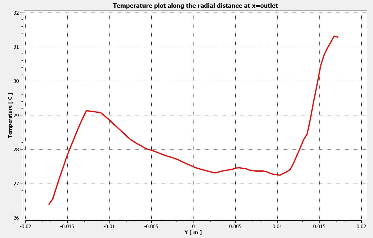
Temperature plot along the radial distance at the outlet:
k-epsilon model:
k-omega SST model:
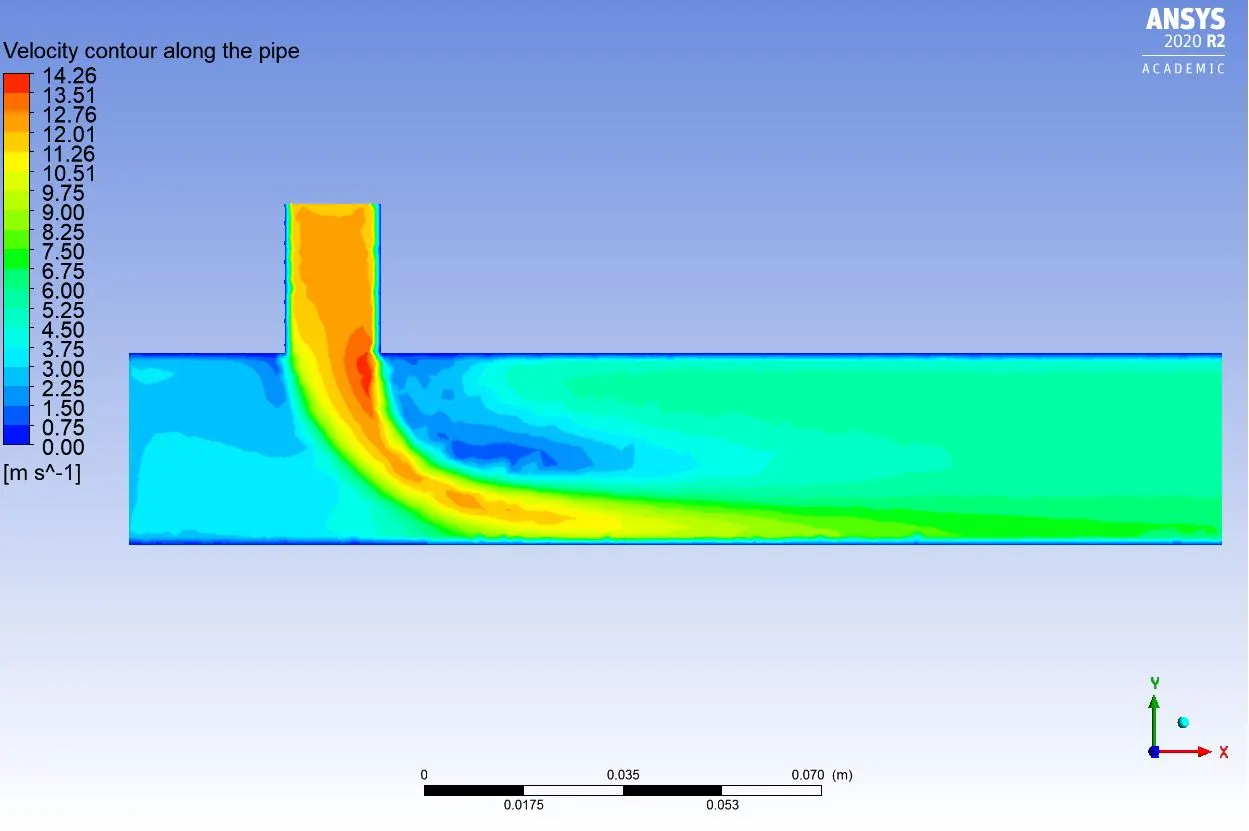
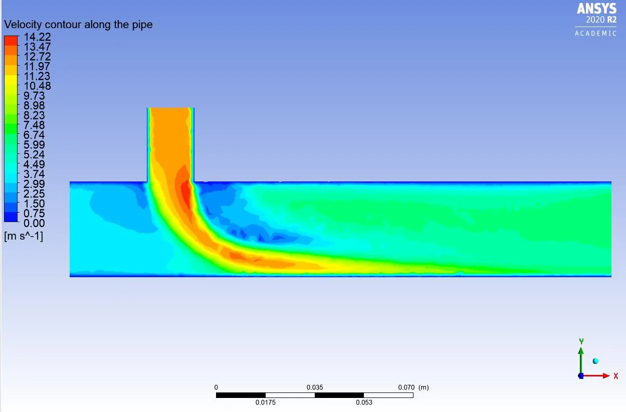
Velocity contour along the pipe:
k-epsilon model:
k-omega SST model:
Velocity plot along the pipe from x=-0.08 to x=0.12:
k-epsilon model:
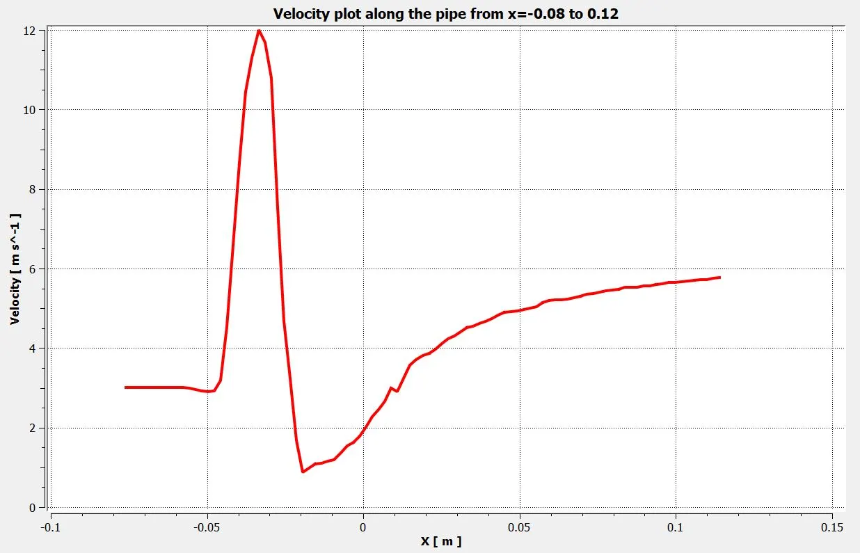
k-omega SST model:
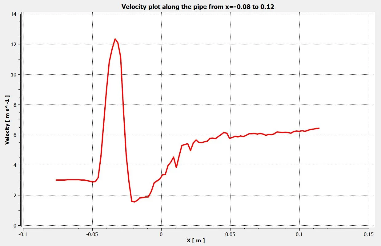
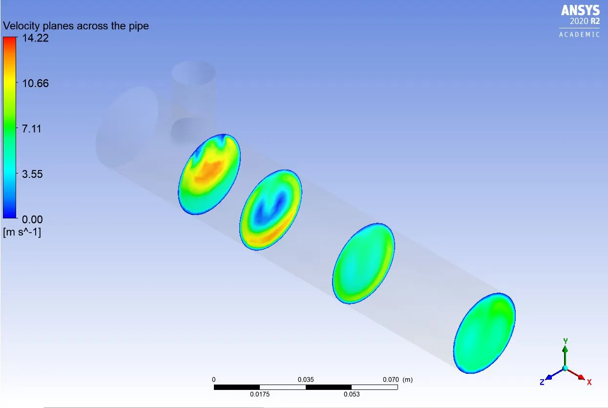
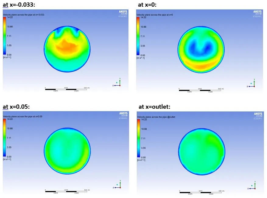
Velocity planes at different distances across the pipe:
k-epsilon model:
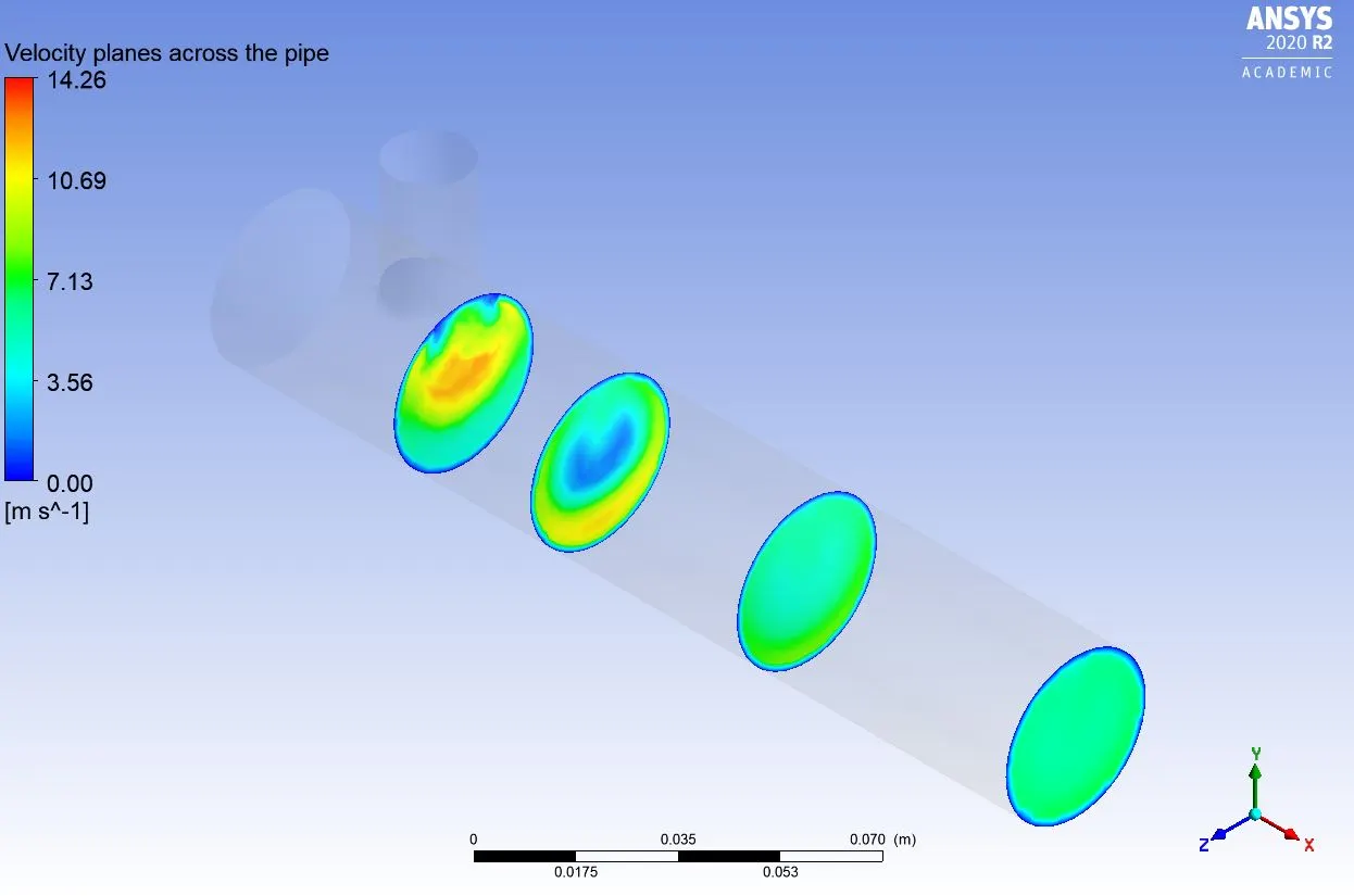
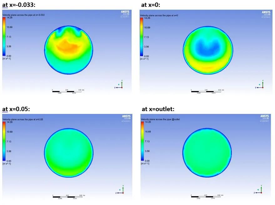
k-omega SST model:
Velocity plot along the radial distance at the outlet:
k-epsilon model:
k-omega SST model:
CONCLUSION:

NOTE: In the above table, the average temperature is calculated at the outlet.
1. From the convergence plot for both k-epsilon and k-omega SST model with momentum ratio 2 and 4, we can observe that, as compared to the k-epsilon model; the k-omega SST model is converging at a larger number of iterations. The possible reason behind that could be the fact that many iterations required to solve the near-wall effects better and the same we can find in further observations related to the k-omega SST model.
2. From standard deviation plots, we can notice that the deviation at the outlet in the k-omega SST model is more than compared to the k-epsilon model. When the momentum ratio is 2, the value of the standard deviation for the k-omega SST model is 2.62 whereas for the k-epsilon model it is 1.85. With momentum ratio=2, the k-epsilon model is much promising in terms of mixing effectiveness of the two fluids. When the momentum ratio is 4, the value of the standard deviation is 1.12 and with the k-epsilon model, we're getting a deviation of 0.78. Since k- epsilon model predicts better far from the boundaries (wall) and k- omega model predicts better near the wall, we're getting values of standard deviation lower in the simulations done with the k-epsilon model. So overall k-epsilon model prediction of mixing effectiveness is better, but by just seeing the values of standard deviation we can not tell which model is performing better than the other without discussing further results.
3. By seeing the different contour plots for both the k-epsilon model and k-omega SST model, it can be observed that the k-omega SST model captures near-wall effect better and when we see the graph of velocity along the radial distance at the outlet, it is worthy to note that both the turbulence models depict velocity profile for the case 1-better. But the k-omega SST model results are in favor because of a more resolved boundary layer near the wall.
4. From the above table we can easily deduce that for both the momentum ratio 2 and 4, the average temperature at the outlet got from the k-omega SST model is much closer to our analytical solution results.
Therefore, from the above observations and discussions, we are sure that the k-omega SST model results are much more promising and better in agreement. So, for further simulations, we are going to use the k-omega SST turbulence model, and also for this setup it is suggested to use the k-omega SST model for better predictions near the wall regions.
Case 2: Long T-junction with a hot inlet velocity of 3m/s and Momentum ratio of 2 & 4
PRE-PROCESSING:
Geometry:
The Long T-junction geometry with units has been shown below and remember that the images shown below are from SolidWorks, and this is not the final geometry we are going to use for simulation.
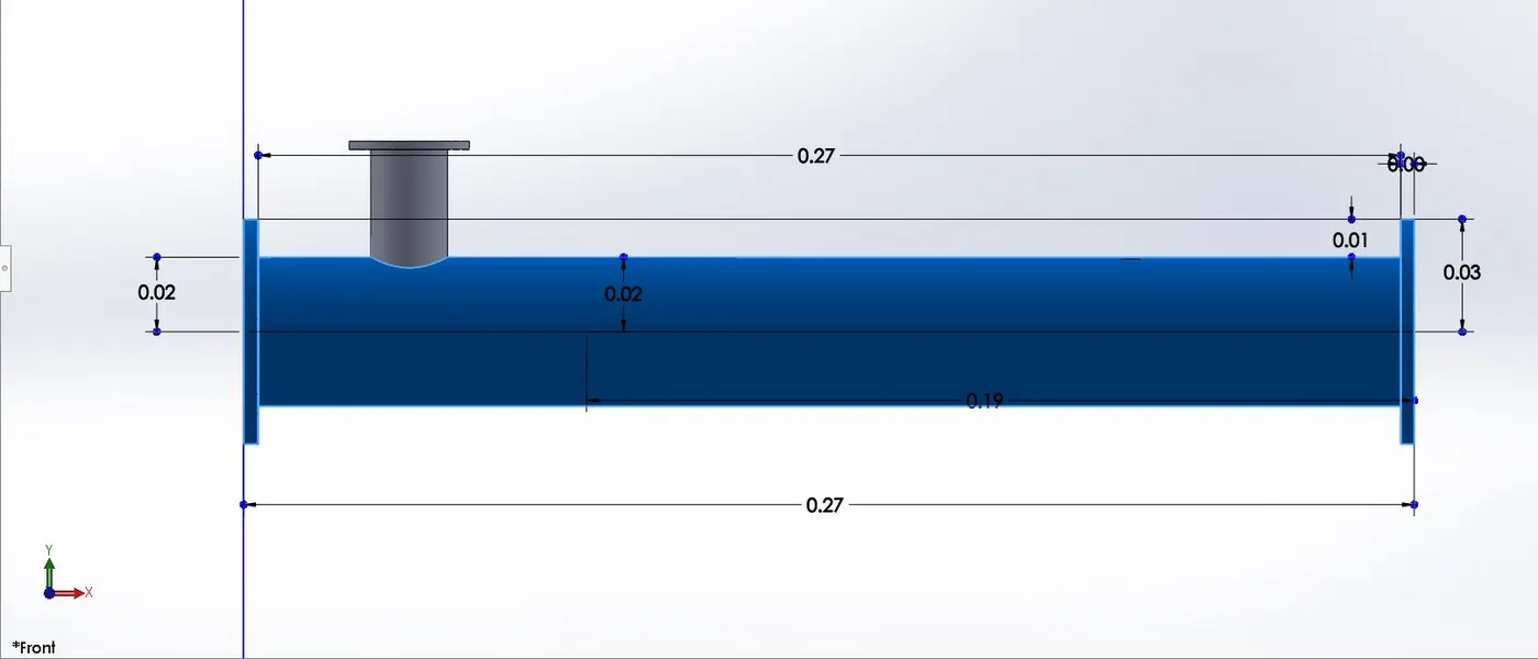
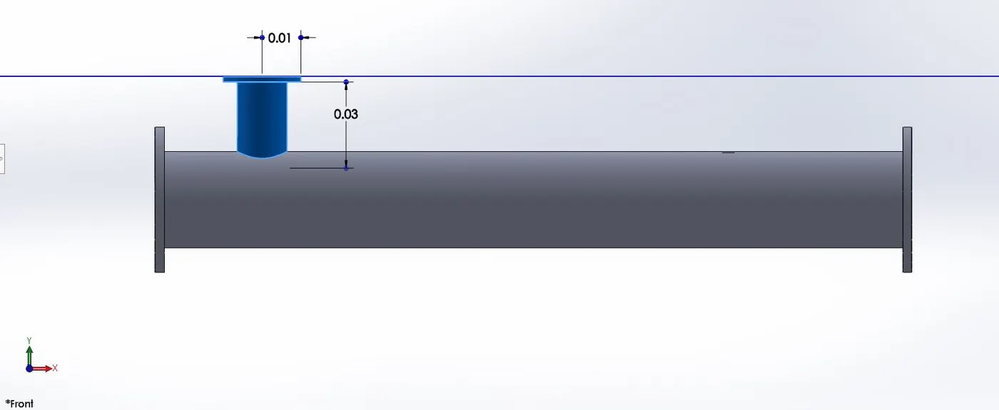
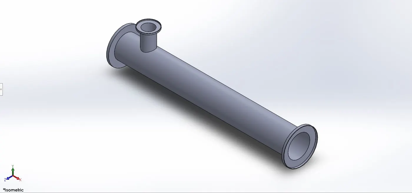
After creating the geometry in SolidWorks, we’ll import the geometry in ANSYS SpaceClaim for the CAD cleaning process. Here in the CAD cleaning process we’ll extract the flow volume field from the model and the extracted volume is shown below:
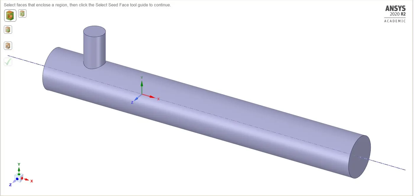
The above geometry is the final long T-junction geometry that we’re going to use in our second case simulation. Hiding the geometry will not affect the object's inclusion in the simulation. To avoid the hidden geometry to be involved in the simulation, use suppress physics option for the solid geometry.
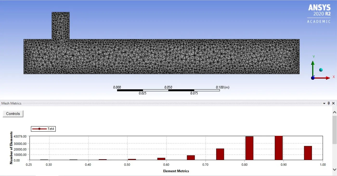
Meshing:
We use ANSYS inbuilt Meshing tool for the discretization of our flow domain for solving. As discussed earlier also, for a better result and good prediction for near-wall calculations we’ll use a fine mesh (element size=2e-003m).
Fine Mesh: element size=2e-003m
Solver Settings:
ANSYS Fluent is used to set up the flow conditions. Here we apply different boundary conditions, like for inlet, outlet, and wall boundary conditions. For initialization, we’ll use ‘Hybrid initialization’.
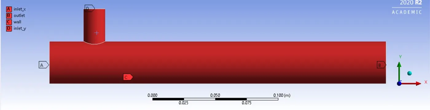
Boundary conditions for inlet, outlet, and wall are:
a) For momentum ratio=2:
inlet_x (hot inlet): velocity=3m/s; temperature=C
Inlet_y (cold inlet): velocity=6m/s; temperature=C
outlet: pressure= 0Pa
wall: no-slip condition
b) For momentum ratio=4:
inlet_x (hot inlet): velocity=3m/s; temperature=C
Inlet_y (cold inlet): velocity=12m/s; temperature=C
outlet: pressure= 0Pa
wall: no-slip condition
Since in our first case we have already seen that the results are in the favor of k-omega SST model and the predictions of k-omega SST model are closer to the analytical solution as compared to the k-epsilon model. Therefore, for our second case, we’ll setup our simulation using k-omega SST model.
Snippets for different solver settings are shown below:
k-omega SST model settings:
NOTE: Don’t forget to check the energy option in the physical settings box before proceeding for hybrid initialization. Also, the number of iterations completely depends on the convergence of the solution, and here we are taking a different numbers of iterations for different simulations. We’ll run a particular simulation until we reach a converged solution and remember that the runtime will differ from simulation to simulation.
POST-PROCESSING:
Results and Discussions for Case 2: (using the k-omega SST turbulence model)
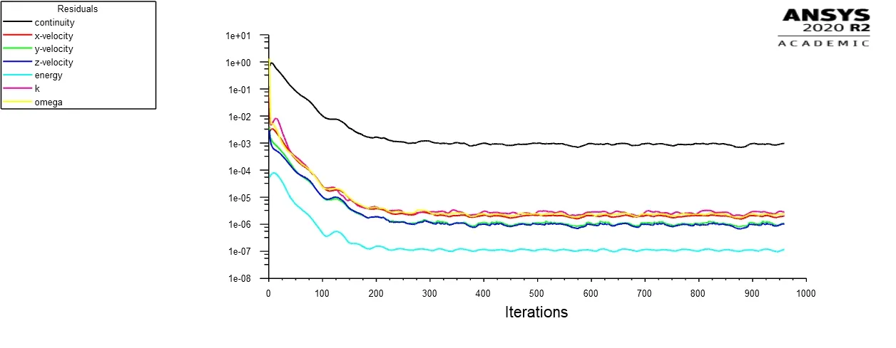
Residual plot:
momentum ratio=2
momentum ratio=4
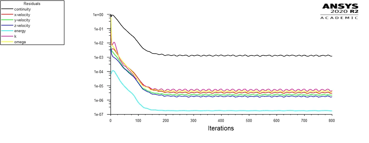
From the above plot of residuals, we can observe that the solution for the k-epsilon model converges near 250 iterations, whereas the k-omega SST model converges near 450 iterations.
Plot for Area-Weighted Average of temperature at the outlet:
momentum ratio=2
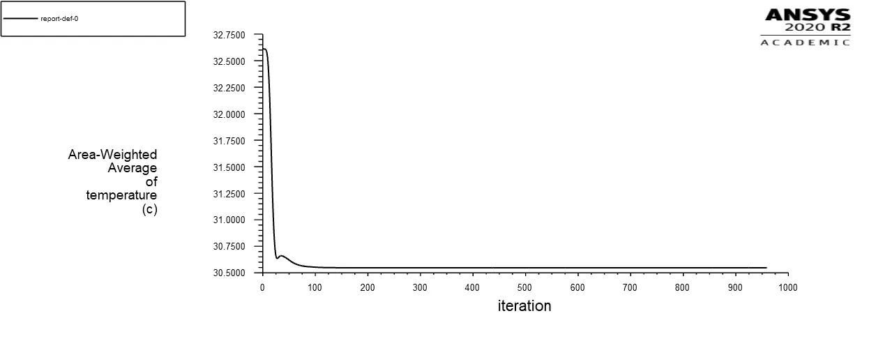
momentum ratio=4
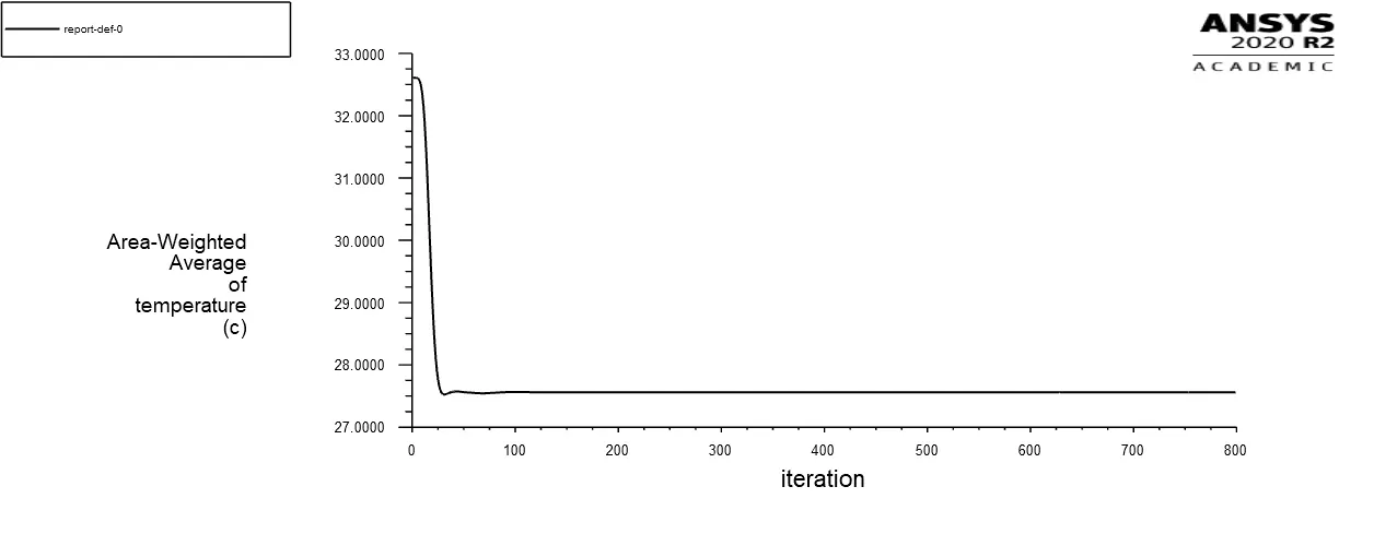
Plot for Standard Deviation of temperature at the outlet:
momentum ratio=2
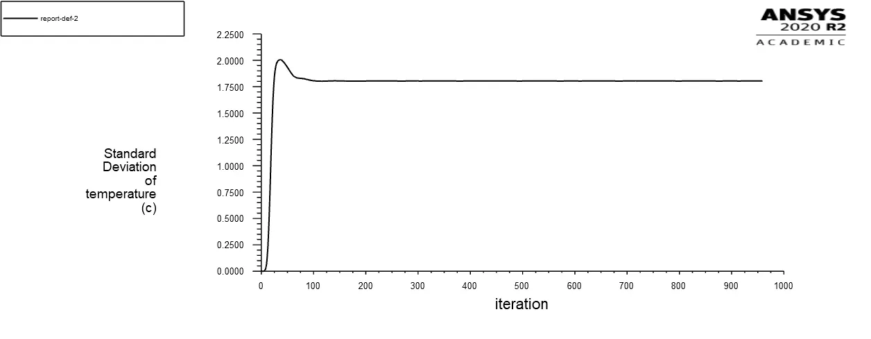
momentum ratio=4
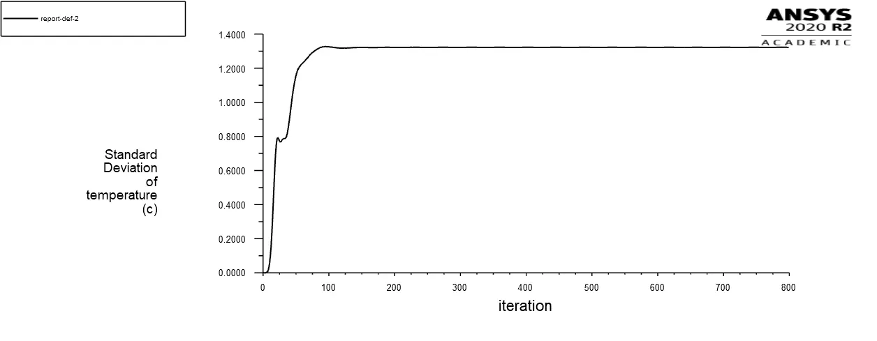
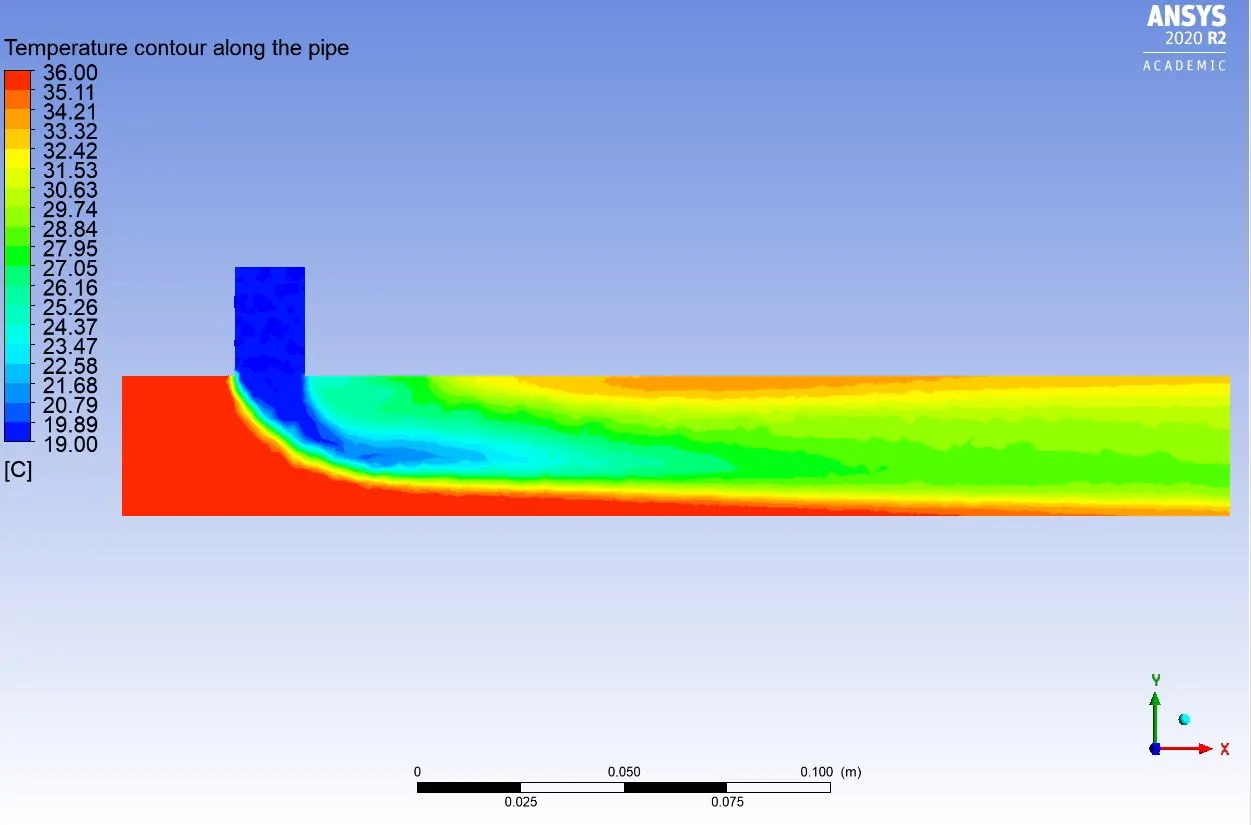
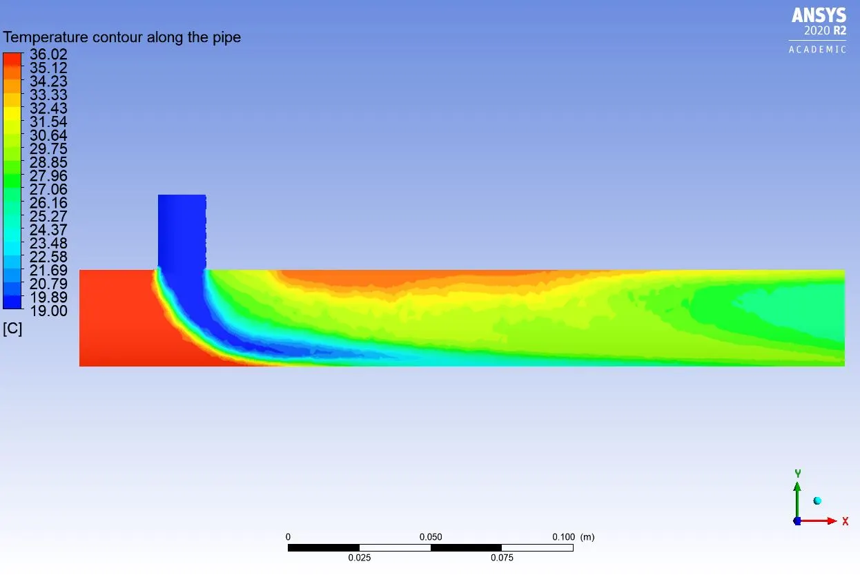
Temperature contour along the pipe:
momentum ratio=2
momentum ratio=4
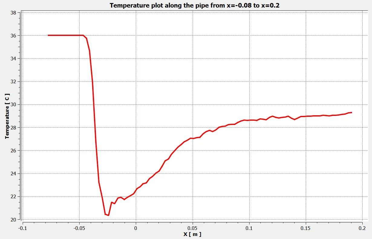
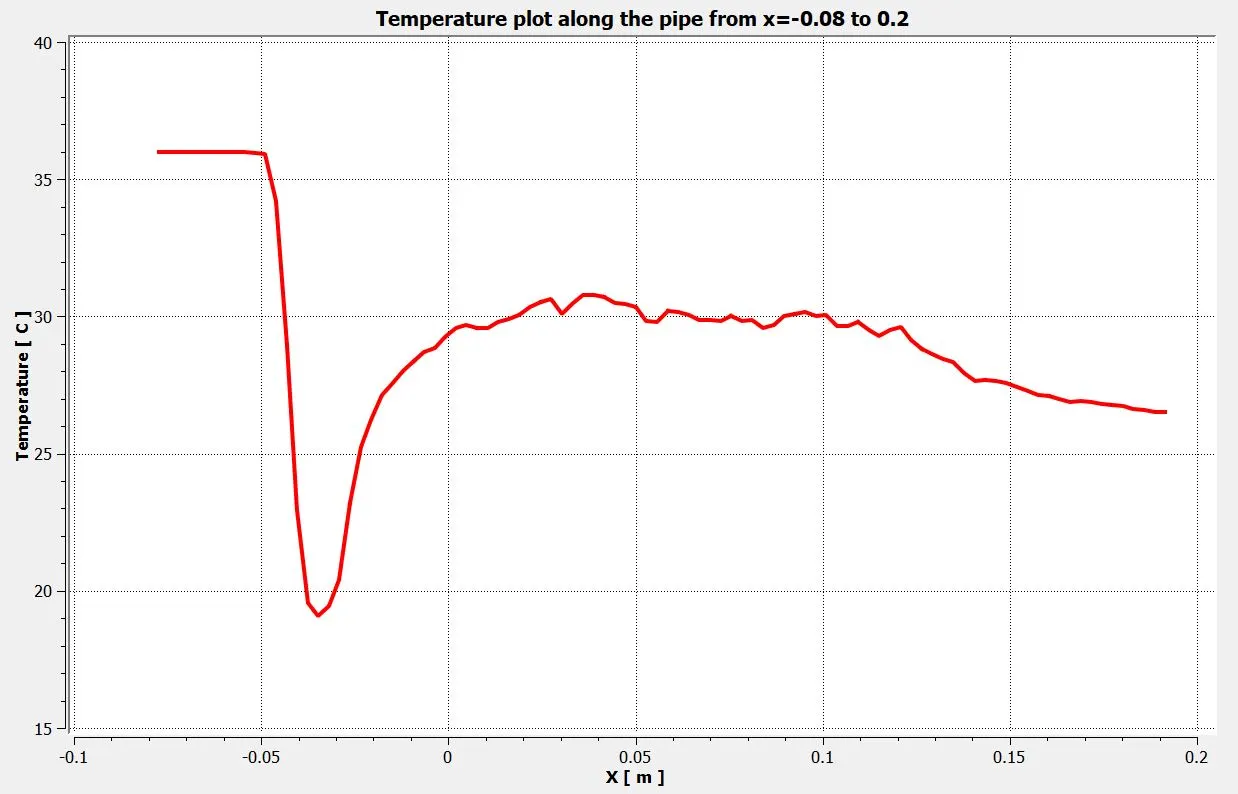
Temperature plot along the pipe from x=-0.08 to x=0.12:
momentum ratio=2
momentum ratio=4
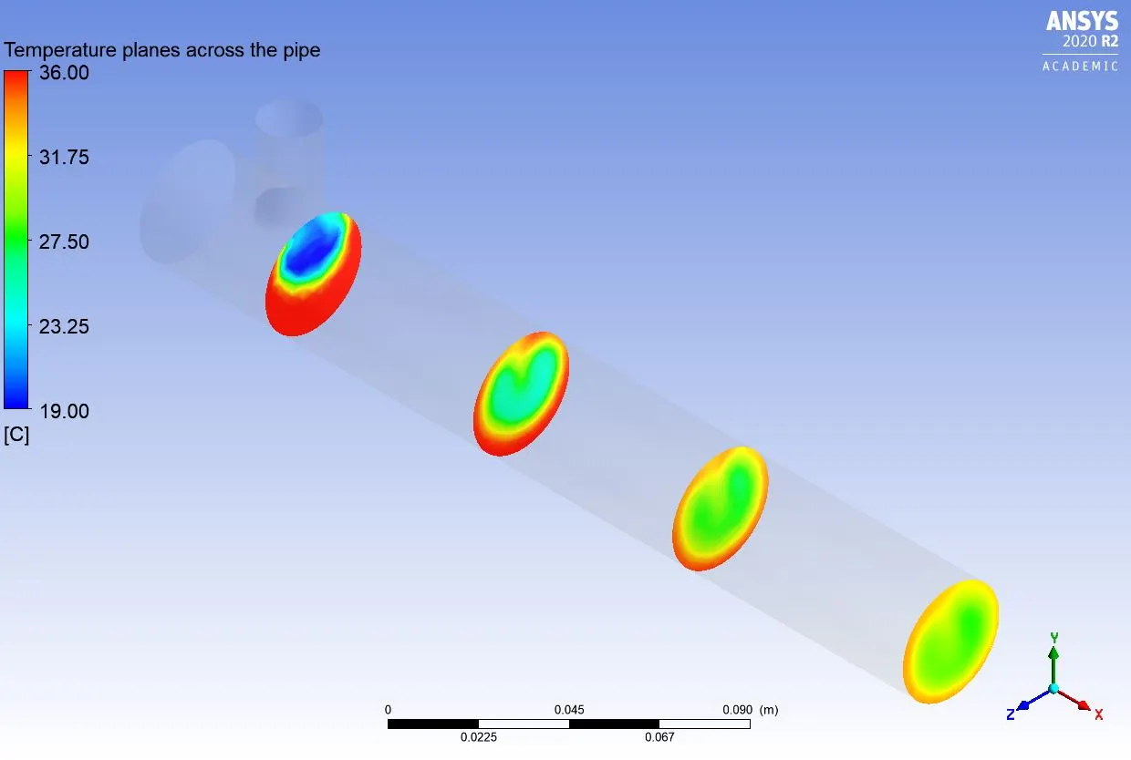
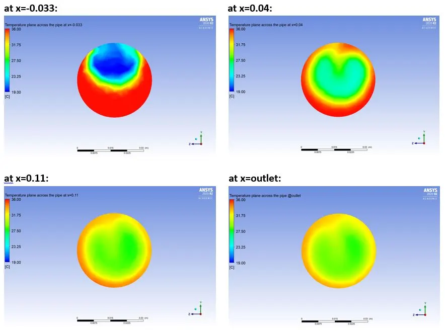
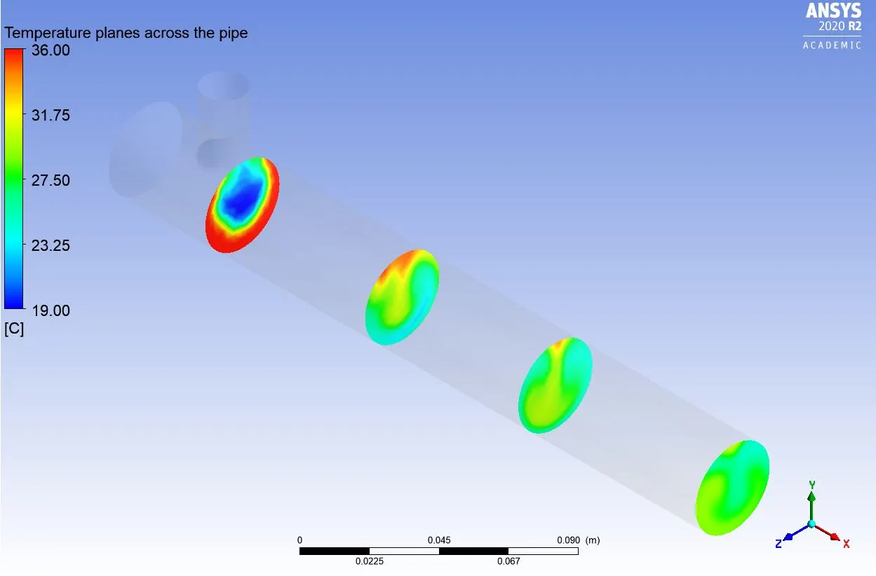
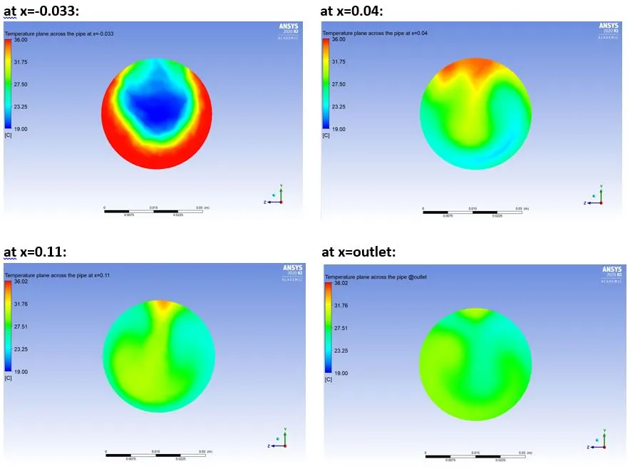
Temperature planes at different distances across the pipe:
momentum ratio=2
momentum ratio=4
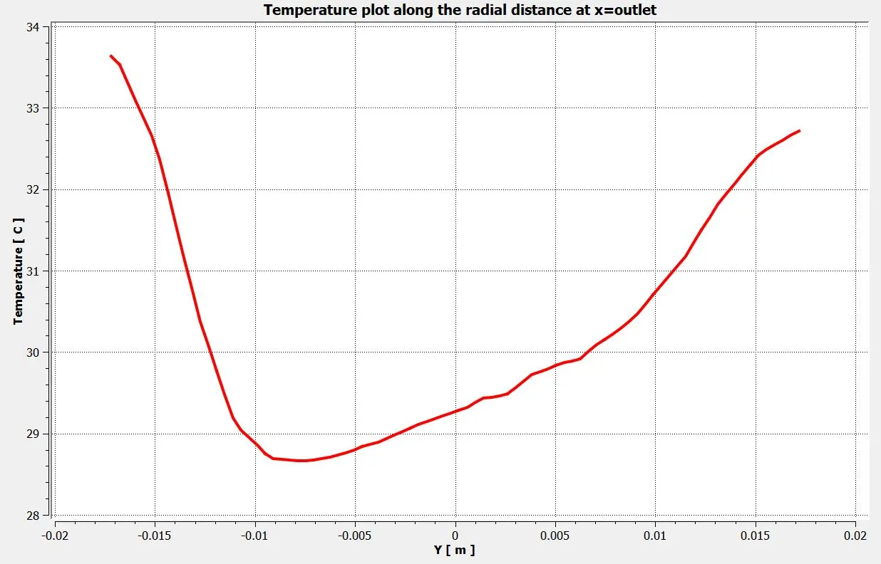
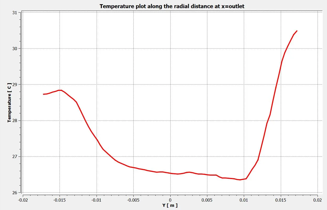
Temperature plot along the radial distance at the outlet:
momentum ratio=2
momentum ratio=4
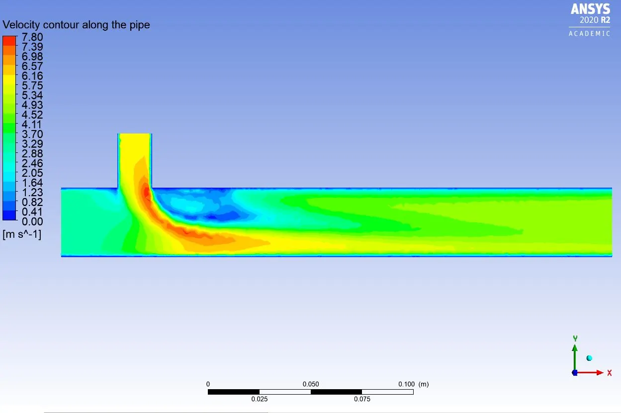
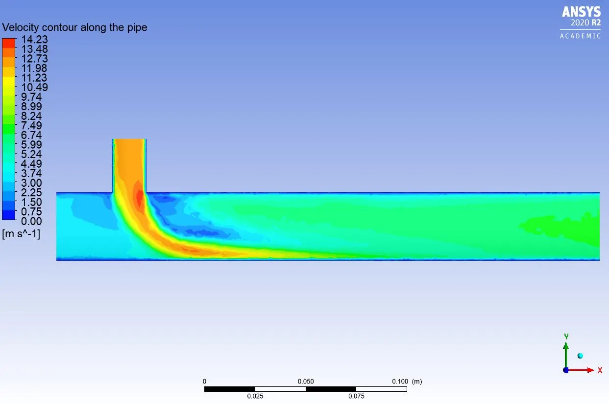
Velocity contour along the pipe:
momentum ratio=2
momentum ratio=4
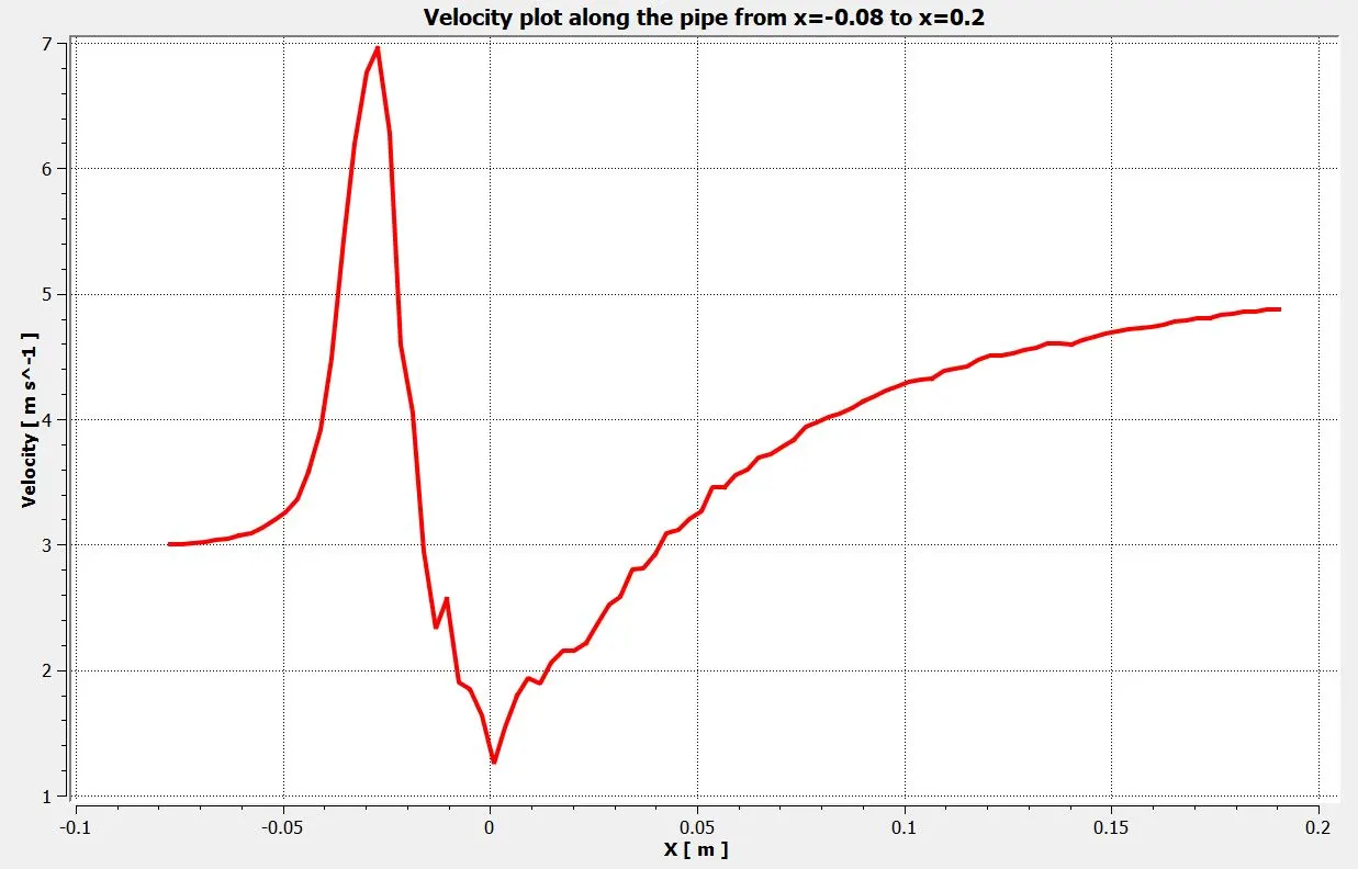
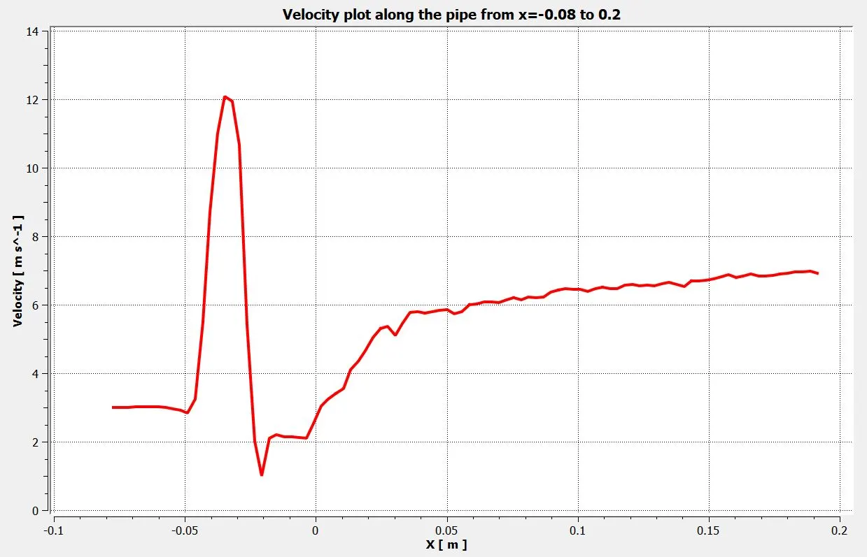
Velocity plot along the pipe from x=-0.08 to x=0.12:
momentum ratio=2
momentum ratio=4
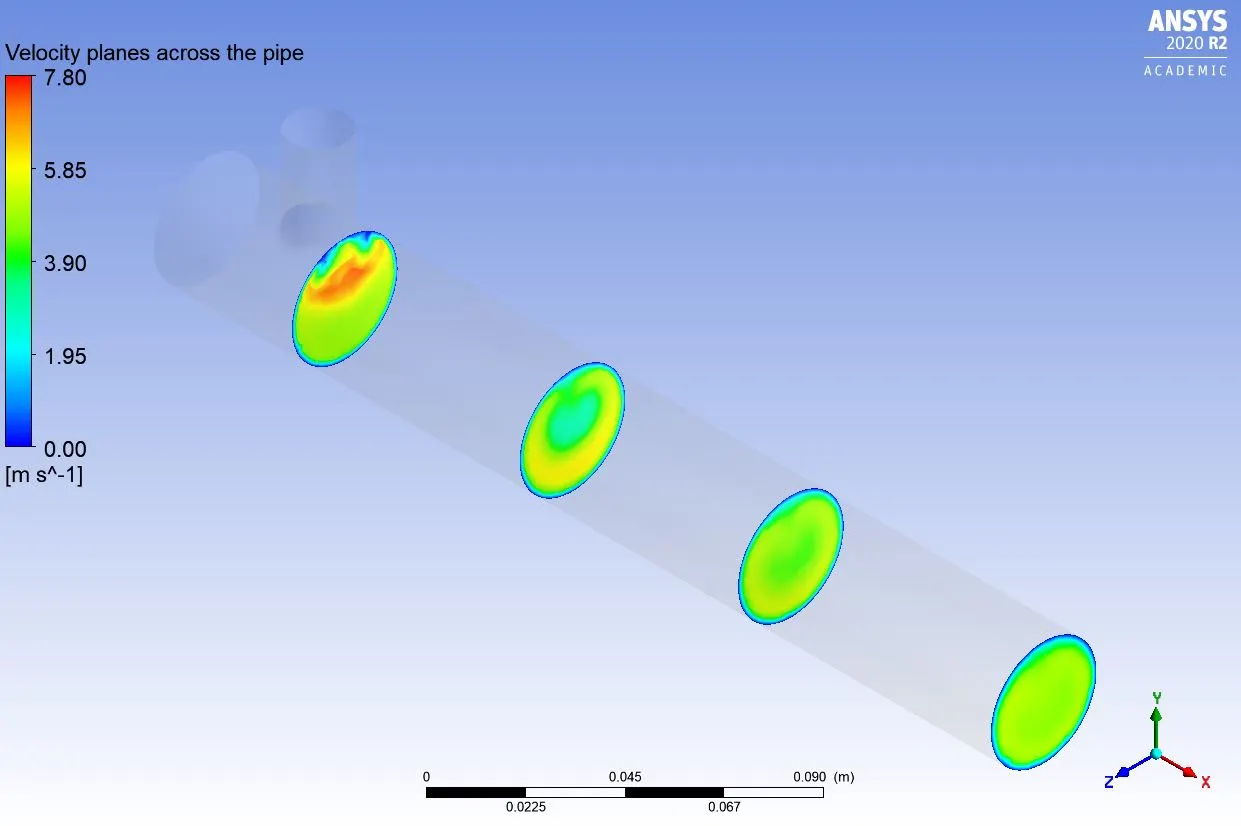
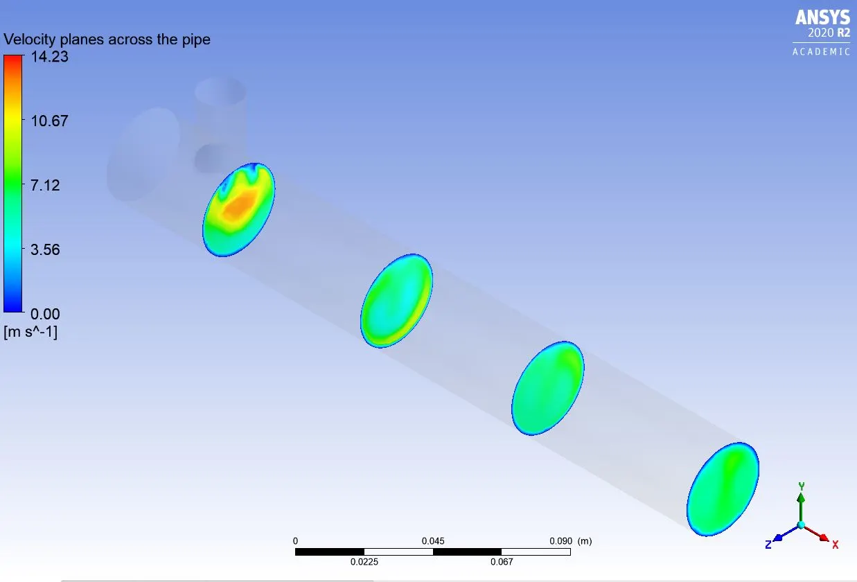
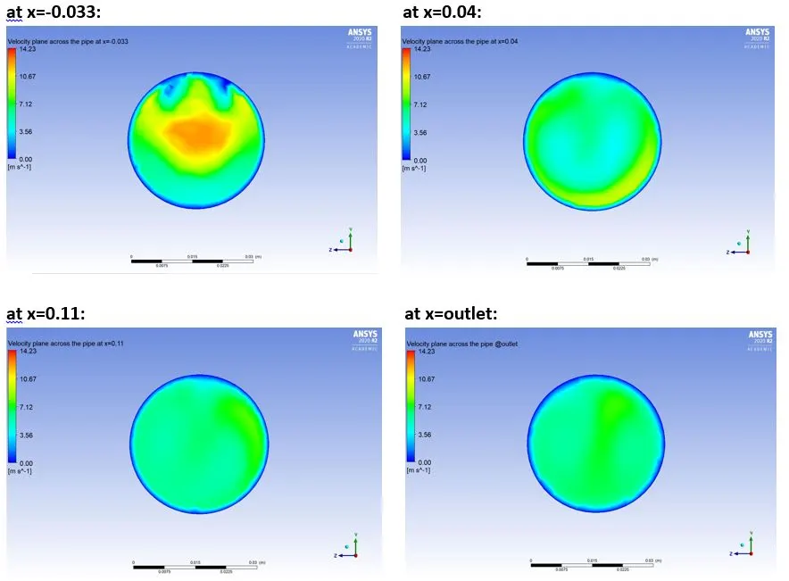
Velocity planes at different distances across the pipe:
momentum ratio=2
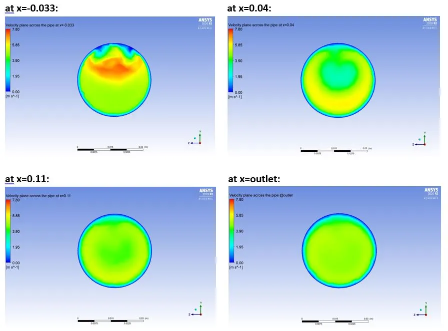
momentum ratio=4
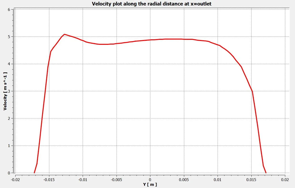
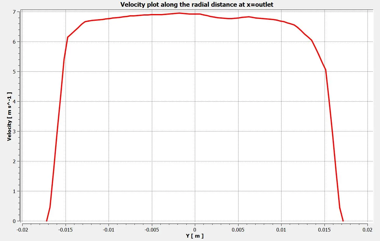
Velocity plot along the radial distance at the outlet:
momentum ratio=2
momentum ratio=4
CONCLUSION:

NOTE: In the above table, the average temperature is calculated at the outlet.
1. We know that a high standard deviation means mixing is bad, whereas a low standard deviation in curve means mixing is good. When the momentum ratio is 2, for short T-junction and long T-junction the value of standard deviation is 2.62 and 1.80 respectively. Whereas when the momentum ratio is 4, the value of standard deviation for short T-junction and long T-junction is 1.12 and 1.32 respectively. So, here we can see that when the momentum ratio is 2, the long T-junction mixing efficiency is better than the short T-junction; but when we increase the momentum ratio to 4, the standard deviation value we get for short T-junction is lower than long T-junction. This means that when we increase our momentum ratio (i.e. increasing the inlet velocity of cold fluid) the mixability in the short T-junction gets better than the long T-junction.
Also, it is noticeable that when we increase the momentum ratio (i.e. the inlet velocity of cold fluid), the mixing efficiency is also increasing.
2. From the contours of temperature in short T-junction with a momentum ratio of 2, it is worthy to observe that the temperature distribution at the outlet is not uniform and some hot air persists because of the uneven mixing of hot air and cold air. Whereas for long T-junction with the same momentum ratio, the mixing of air is more uniform than the short T-junction and also the average temperature at the outlet has been decreased.
3. From the contours of temperature in short and long T-junctions with a momentum ratio of 4, we can notice a drop in average temperature at the outlet and that is because of the increase in the inlet velocity of cold air. Also, we can see that the error percentage in the short T-junction with the momentum ratio of 4 is less than the long T-junction with the same momentum ratio. By this we can conclude that the inlet velocity of cold air is the dominant factor in determining the outlet conditions.
4. The temperature contour at the outlet for short T-junction cases shows that some high temperatures flow sips through without properly mixing with the flow. Whereas, in the temperature contour of long tee cases, the high temperatures flow thoroughly mixes with the rest of the flow. From the above table we can conclude that for uniform mixing of air, the long T-junction is recommended whereas the outlet temperature can be reduced by increasing the velocity of cold inlet air while keeping the length of T-junction constant.