Simulation of a 1D Super-sonic nozzle flow simulation using Macormack Method

Aim:

To conduct the simulation of a 1D super-sonic nozzle flow simulation using Macormack method in MATLAB.

Objectives:

• To simulate the isentropic flow through a quasi 1D subsonic-supersonic nozzle.
• To conduct the simulation by conservative and non conservative methods.
• To analyse the plots of steady-state distribution of primitive variables inside the nozzle.
• To analyse the plots of time-wise variation of the primitive variables.
• To analyse the variation of Mass flow rate distribution inside the nozzle at different time steps during the time-marching process.
• To made a comparison of Normalized mass flow rate distributions of both forms.
• To conduct grid dependency test.

Nozzle flow:

An isentropic nozzle is considered in the project. This nozzle consists of convergent section, throat and the divergent section. The convergent section has a huge cross sectional area, therefore the velocity at the convergent section is minimum. The density,pressure and temperature at the entry of the convergent section is defined as `rho0`,`P0` and `T0`. The throat region has the minimal area when compared with convergent and divergent section.

The Mach number(M) depicts the type of flow happening in the each section of the nozzle. The Mach number is equal to 1 (M=1) at the throat region. The divergent section has a required cross section of area. The Mach number value less tha 1 describes that the flow is subsonic. The Mach number value equal to 1 describes that the flow is sonic in nature. The Mach number value greater than 1 indicates that the flow is supersonic. The area, pressure and temperature at the throat region is denoted as A',P' and T'. The divergent region is mostly a supersonic region. The pressure, temperature, velocity and mach number at the divergent region is denoted as `P_e`,`T_e`,`V_e` and `M_e`.

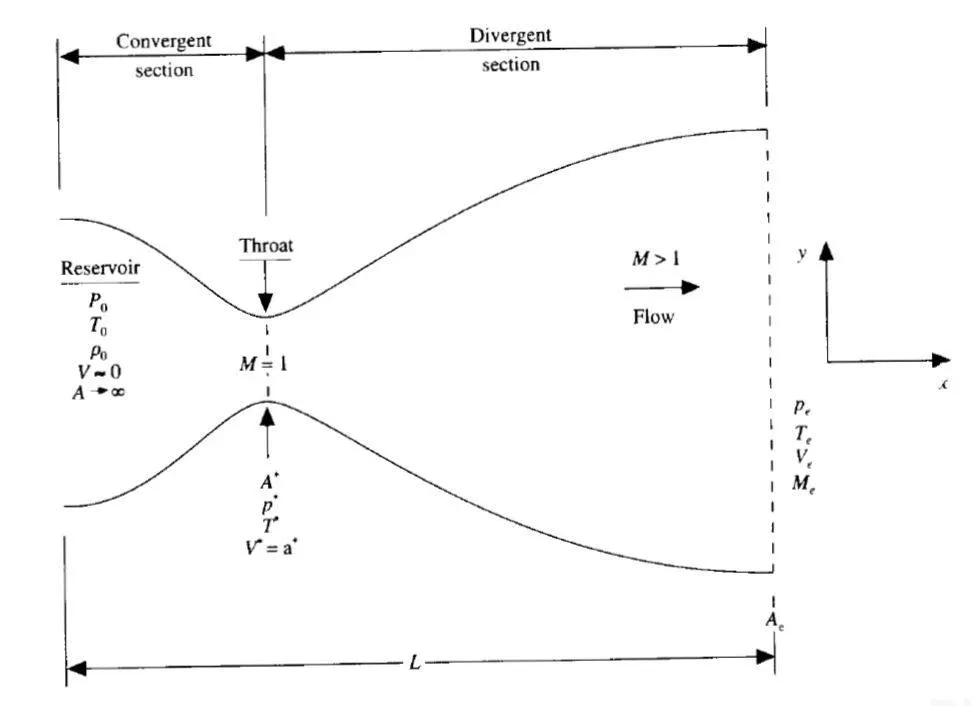
The governing equation for two different method was derived individually and they are solved using macormack method.

Non-conservative method:

The governing equation including continuity, momentum and energy equation of non-conservative method was derived.

Governing equations:

Continuity equation - `rho_1*V_1*A_1 = rho_2*A_2*V_2`

Momentum equation - `p_1*A_1+rho_1*V_1^2*A_1+int_(A1)^(A2)p*dA = p_2*A_2+rho_2*V_2^2*A_2`

Energy equation - `h_1+(V_1^2/2) = h_2+(V_2^2/2)`

These equations are solved using macormack method. The three type of governing equations are simplified or solved for one dimensional quasi supersonic nozzle flow. Inorder to convert this, a control volume is assumed and the flow parameters are derived at that control volume.

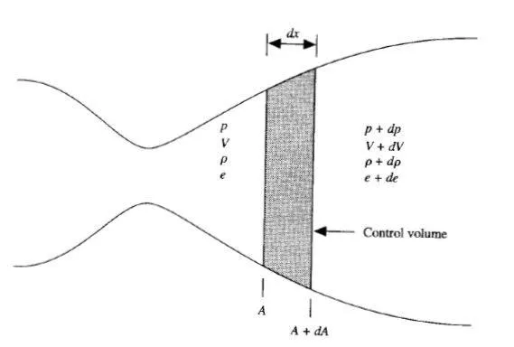
Finally, the governing equation for the 1D quasi supersonic nozzle flow is obtained as,

Continuity equation - `(delrho^')/(delt') = -rho'((delV')/(delx'))-rho'V'((del(ln A'))/(delx'))-V'((delrho')/(delx'))`

Momentum equation - `(delV')/(delt') = -V'((delV')/(delx'))-(1/gamma)((delT')/(delx')+((T')/(rho'))((delrho')/(delx')))`

Energy equation - `(delT')/(delt') = -V'((delT')/(delx'))-(gamma-1)T'[(delV')/(delx')+V'((del(ln A'))/(delx'))]`

where the density, temperature and pressure ratio were found from the general term as,

`P/P_0=(1+(gamma-1)/2(M^2))^(-gamma/(gamma-1))`

`rho/rho_0 = (1+(gamma-1)/2(M^2))^(-1/(gamma-1))`

`T/T_0 = (1+(gamma-1)/2(M^2))^-1`

The three governing equations are solved using macormack method under various steps.

Macormack method and discretization:

The macormack method is a method in which time marching solutions are obtained. The macormack method consists of two steps to solve the governing equations. They are predictor method and the corrector method. Initially, the grid points are assigned. With the help of assigned initial values, the parameters at the successive nodes are found by using forward and backward differencing approaches. In the predictor step, the governing equations are solved using forward differencing scheme. After this step, the solutions are get updated. Then, the corrected step uses the backward differencing scheme for solving the governing equations. Final solutions are updated and plotted. Since it is a 1D problem a line passed through the centre of the nozzle is considered and the nodes are assigned on that line.

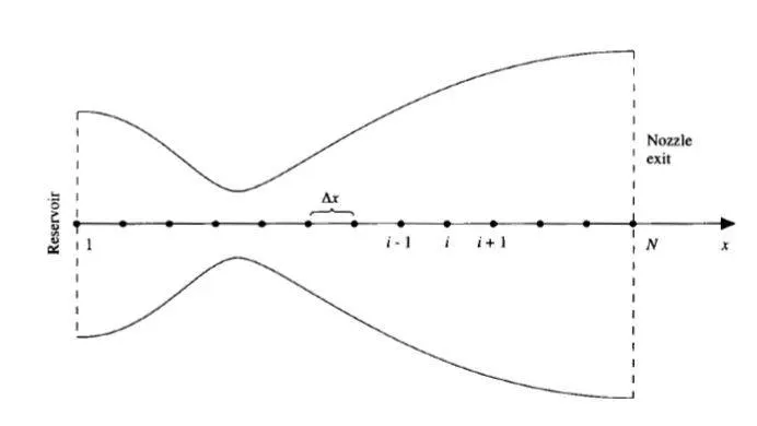
Initial and boundary conditions:

The initial profile of density, temperature and the velocity is assigned by the following formulae,

`rho = 1-0.3146*x`

`T = 1-0.2314*x`

`V = (0.1+1.09*x)sqrtT`

The different boundary conditions at the inlet and the outlet of the nozzle is asssigned.

At inlet of the nozzle, the velocity boundary condition is assigned. At the outlet of the nozzle, the density, velocity and the temperature values are assigned.

MATLAB code (Non conservative function):

function[rho,v,t,rho_th,v_th,t_th,P_th,Ma_th,m_th,mn]=non_conservative(n,x,dx,gamma,Area)

%Initial profiles
rho = 1-0.3146*x;
t = 1-0.2314*x;
v = (0.1+1.09*x).*t.^0.5;

%Throat region
Th = (n+1)/2;

%Time step 
nt = 1000;

%dt calculation
C = 0.5;
for i=1:n
    A = t.^0.5;
    dt(i) = C*(dx/(A(i)+v(i)));
end
dt = min(dt);

%Outer time loop
for j=1:nt
        
    rho_old = rho;
    v_old = v;
    t_old = t;
    
    %Predictor step

    for k=2:n-1
        dvdx = (v(k+1)-v(k))/dx;
        drhodx = (rho(k+1)-rho(k))/dx;
        dtdx = (t(k+1)-t(k))/dx;
        dlogadx = (log(Area(k+1))-log(Area(k)))/dx;
        
        %Continuity equation
        drhodt_p(k) = -rho(k)*dvdx-rho(k)*v(k)*dlogadx-v(k)*drhodx;
        
        %Momentum equation
        dvdt_p(k) = -v(k)*dvdx-(1/gamma)*(dtdx + (t(k)/rho(k))*drhodx);
        
        %Energy equation
        dtdt_p(k) = -v(k)*dtdx-(gamma-1)*t(k)*(dvdx + v(k)*dlogadx);
        
        %Solution update
        rho(k) = rho(k) + drhodt_p(k)*dt;
        v(k) = v(k) + dvdt_p(k)*dt;
        t(k) = t(k) + dtdt_p(k)*dt;
        
    end
    
    %Corrector step

    for k=2:n-1
        dvdx = (v(k)-v(k-1))/dx;
        drhodx = (rho(k)-rho(k-1))/dx;
        dtdx = (t(k)-t(k-1))/dx;
        dlogadx = (log(Area(k))-log(Area(k-1)))/dx;
        
        %Continuity equation
        drhodt_c(k) = -rho(k)*dvdx-rho(k)*v(k)*dlogadx-v(k)*drhodx;
        
        %Momentum equation
        dvdt_c(k) = -v(k)*dvdx-(1/gamma)*(dtdx + (t(k)/rho(k))*drhodx);
        
        %Energy equation
        dtdt_c(k) = -v(k)*dtdx-(gamma-1)*t(k)*(dvdx + v(k)*dlogadx);
        
    end
    
    %Average time derivative
    drhodt = 0.5*(drhodt_p+drhodt_c);
    dvdt = 0.5*(dvdt_p+dvdt_c);
    dtdt = 0.5*(dtdt_p+dtdt_c);
    
    %Final solution update
    for i=2:n-1
      rho(i) = rho_old(i) + drhodt(i)*dt;
      v(i) = v_old(i) + dvdt(i)*dt;
      t(i) = t_old(i) + dtdt(i)*dt;
    end
    
    %Boundary condition
    %Inlet
    v(1) = 2*v(2)-v(3);
    
    %Outlet
    rho(n) = 2*rho(n-1)-rho(n-2);
    v(n) = 2*v(n-1)-v(n-2);
    t(n) = 2*t(n-1)-t(n-2);
    
    %Pressure
    P = rho.*t;
    %Mass
    mn= rho.*Area.*v;
    %Mach number
    Ma = v./(sqrt(t));
    
    %Parameters at the throat region
    rho_th(j) = rho(Th);
    v_th(j) = v(Th);
    t_th(j) = t(Th);
    P_th(j) = P(Th);
    Ma_th(j) = Ma(Th);
    m_th(j) = mn(Th);
    
    %Plotting
    
    %Instantaneous distributions of the nondimensional mass flow as a function of distance
    %Non dimensional distance vs mass flow rate
    figure(1)
    hold on
      if j == 50
          plot(x,mn,'k')
      elseif j == 100
          plot(x,mn,'r')
      elseif j == 150
          plot(x,mn,'b')
      elseif j == 200
          plot(x,mn,'g')
      elseif j == 700
          plot(x,mn,'y')
          legend('50 dt','100 dt','150 dt','200 dt','700 dt')
          xlabel('Non dimensional distance (x)')
          ylabel('Non dimensional mass flow')
          title('Instantaneous distributions of the nondimensional mass flow as a function of distance')
      end
          
end 
    %Plotting
    
    %Qualitative aspects of quasi-one-dimensional nozzle flow
    figure(2)
    subplot(4,1,1)
    %Non dimensional distance vs Mach number
    plot(x,Ma,'k')
    ylabel('Mach Number')
    subplot(4,1,2)
    %Non dimensional distance vs Pressure ratio
    plot(x,P,'r')
    ylabel('Pressure ratio')
    subplot(4,1,3)
    %Non dimensional distance vs Density ratio
    plot(x,rho,'b')
    ylabel('Density ratio')
    subplot(4,1,4)
    %Non dimensional distance vs Temperature ratio
    plot(x,t,'g')
    ylabel('Temperature ratio')
    xlabel('X')
    
    %Timewise variations of the density, temperature, pressure, and Mach number at the nozzle throat
    figure(3)
    subplot(4,1,1)
    %Timestep vs density ratio
    plot(rho_th,'k')
    ylabel('rho/rho0')
    subplot(4,1,2)
    %Timestep vs temperature ratio
    plot(t_th,'r')
    ylabel('T/T0')
    subplot(4,1,3)
    %Timestep vs Pressure ratio
    plot(P_th,'b')
    ylabel('p/p0')
    subplot(4,1,4)
    %Timestep vs Mach number
    plot(Ma_th,'g')
    ylabel('Mach number')
    xlabel('Time step')
    
    figure(7)
    plot(x,mn)
    title('Non dimensional distance vs Mass flow rate')
    xlabel('Non dimensional distance (x)')
    ylabel('Mass flow rate (m)')
    
    
end

Code explanation:

• The input values such as number of nodes(n), area and other parameters are assigned on the main program.
• The initial profile and the time step values are assigned.
• The "dt" value is found by using the formula `dt = C*(dx/(sqrtT+V))`
• The outer time loop is opened and the initial set of values are assigned.
• The predictor method is solved inside a for loop and the solution is updated.
• The correcteor method is solved and the final solution is updated inside a specific for loop.
• The various parameters are decoded and the values at the throat is obtained.
• The results are plotted and analysed.

Conservative method:

The governing equation including continuity, momentum and energy equation of non-conservative method was derived.

Governing equations:

Continuity equation - `(del(rho'A'))/(delt')+(del(rho'A'V'))/(delx')`

Momentum equation - `(del(rho'A'V'))/(delt)+((del[rho'A'V'^2+(1/gamma)p'A'])/(delx'))=(1/gamma)p'(delA')/(delx')`

Energy equation - `(del[rho'((e')/(gamma-1)+(gamma/2)V'^2)A'])/(delt')+(del[rho'((e')/(gamma-1)+(gamma/2)V'^2)V'A'+p'A'V'])/(delx')=0`

These equations are solved using macormack method. These equations are further solved with the help of assigning various factors and flux factors. They are simplified using the following factors,

`U_1 = rho'A'`

`U_2 = rho'A'V'`

`U_3 = rho'((e')/(gamma-1)+(gamma/2)V'^2)A'`

`F_1 = rho'A'V'`

`F_2 = rho'A'V'^2+(1/gamma)p'A'`

`F_3 = rho'((e')/(gamma-1)+(gamma/2)V'^2)V'A'+p'A'V'`

`J_2 = (1/gamma)p'((delA')/(delx'))` with the help of these factors the governing equations are further simplified as,

Continuity equation - `(delU_1)/(delt')=-(delF_1)/(delx')`

Momentum equation - `(delU_2)/(delt')=-(delF_2)/(delx')+J_2`

Energy equation - `(delU_3)/(delt')=-(delF_3)/(delx')`

The final values of `F_1`,`F_2` and `F_3` are,

`F_1 = U_2`

`F_2 = (U_2^2)/(U_1)+(gamma-1)/(gamma)(U_3-(gamma/2)(U_2^2)/(U_1))`

`F_3 = gamma(U_2U_3)/U_1-((gamma)(gamma-1))/2(U_2^3)/U_1^2`

Macormack method and discretization:

The macormack method is a method in which time marching solutions are obtained. The macormack method consists of two steps to solve the governing equations. They are predictor method and the corrector method. Initially, the grid points are assigned. With the help of assigned initial values, the parameters at the successive nodes are found by using forward and backward differencing approaches. In the predictor step, the governing equations are solved using forward differencing scheme. After this step, the solutions are get updated. Then, the corrected step uses the backward differencing scheme for solving the governing equations. Final solutions are updated and plotted.

Initial and boundary condition:

The initial profile of density and temperature for the conservative form is assigned as,

`rho' = 1.0;T'=1.0}`for`0<=x'<=0.5`

`rho'=1.0-0.366(x'-1.5); T'=1.0-0.167(x'-0.5)}`for`0.5<=x'<=1.5`

`rho'= 0.634-0.3879(x'-1.5); T'=0.833-0.3507(x'-1.5)}`for`1.5<=x'<=3.5`

The `U_1,U_2`and `U_3` inlet boundary conditions are assigned along with velocity condition. Similarly at the outlet the `U_1,U_2` and `U_3` values are assigned.

MATLAB code (conservative function):

function[rho,v,t,rho_th,v_th,t_th,P_th,Ma_th,m_th,mc]=conservative(n,x,dx,gamma,Area)

%Initial profiles
for i=1:n
    if x(i)>=0&&x(i)<=0.5
        rho(i) = 1;
        t(i) = 1;
    elseif x(i)>=0.5&&x(i)<=1.5
        rho(i) = 1-0.366*(x(i)-0.5);
        t(i) = 1-0.167*(x(i)-0.5);
    elseif x(i)>=1.5&&x(i)<=3.5
        rho(i) = 0.634-0.3879*(x(i)-1.5);
        t(i) = 0.833-0.3507*(x(i)-1.5);
    end
    v(i) = 0.59/(rho(i)*Area(i));
end

%Throat region
Th = (n+1)/2;

%Time step 
nt = 1000;

%dt calculation
C = 0.5;
for i=1:n
    A = t.^0.5;
    dt(i) = C*(dx/(A(i)+v(i)));
end
dt = min(dt);

%The governing equation is solved using solutions vector U, the flux vector F, and the source term J
%Initial conditions for U1,U2 and U3
U1 = rho.*Area;
U2 = rho.*Area.*v;
U3 = rho.*((t./(gamma-1))+((gamma/2).*(v.^2))).*Area;

%Outer time loop
for j=1:nt
    
    U_old_1 = U1;
    U_old_2 = U2;
    U_old_3 = U3;
    
    %Predictor step
    F1 = U2;
    F2 = ((U2.^2)./U1)+(((gamma-1)/gamma)*(U3-((gamma/2)*((U2.^2)./U1))));
    F3 = ((gamma*U2.*U3)./U1)-(gamma*(gamma-1)*(U2.^3))./(2*(U1.^2));
    
    for k=2:n-1
        
        dadx = ((Area(k+1)-Area(k)))/dx;
        J2 = rho(k)*t(k)*dadx/gamma;
        
        %Continuity equation
        du1dt_p(k) = -(F1(k+1)-F1(k))/dx;
        
        %Momentum equation
        du2dt_p(k) = -(F2(k+1)-F2(k))/dx+J2;
        
        %Energy equation
        du3dt_p(k) = -(F3(k+1)-F3(k))/dx;
        
        %Solution update
        U1(k) = U1(k)+du1dt_p(k)*dt;
        U2(k) = U2(k)+du2dt_p(k)*dt;
        U3(k) = U3(k)+du3dt_p(k)*dt;
    end
    
    v_p = U2./U1;
    rho_p = U1./Area;
    t_p = (gamma-1)*((U3./U1)-((gamma/2)*(v_p.^2)));  
    %Corrector step
    F1 = U2;
    F2 = ((U2.^2)./U1)+(((gamma-1)/gamma)*(U3-((gamma/2)*((U2.^2)./U1))));
    F3 = ((gamma*U2.*U3)./U1)-(gamma*(gamma-1)*(U2.^3))./(2*(U1.^2));

    
    for k=2:n-1
        
        dadx = ((Area(k)-Area(k-1)))/dx;
        J2 = rho_p(k)*t_p(k).*dadx/gamma;
        
        %Continuity equation
        du1dt_c(k) = -(F1(k)-F1(k-1))/dx;
        
        %Momentum equation
        du2dt_c(k) = -(F2(k)-F2(k-1))/dx+J2;
        
        %Energy equation
        du3dt_c(k) = -(F3(k)-F3(k-1))/dx;
        
    end
    
    %Average time derivative
    du1dt = 0.5*(du1dt_p+du1dt_c);
    du2dt = 0.5*(du2dt_p+du2dt_c);
    du3dt = 0.5*(du3dt_p+du3dt_c);
    
    %Final solution update
    for i=2:n-1
        U1(i) = U_old_1(i)+du1dt(i)*dt;
        U2(i) = U_old_2(i)+du2dt(i)*dt;
        U3(i) = U_old_3(i)+du3dt(i)*dt;
    end
    
    %Boundary condition
    %Inlet
    
    U1(1) = rho_p(1).*Area(1);
    U2(1) = 2*U2(2)-U2(3);
    v_p(1) = U2(1)/U1(1);
    U3(1) = U1(1)*((t_p(1)/(gamma-1))+((gamma/2)*v_p(1).*v_p(1)^2));
    
    
    %Outlet 
    
    U1(n) = 2*U1(n-1)-U1(n-2);
    U2(n) = 2*U2(n-1)-U2(n-2);
    U3(n) = 2*U3(n-1)-U3(n-2);
    
    %Density
    rho = U1./Area;
    %velocity
    v = U2./U1;
    %Temperature
    t = (gamma-1).*((U3./U1)-((gamma/2).*(v.^2)));
    %Pressure
    P = rho.*t;
    %Mass
    mc= U2;
    %Mach number
    Ma = v./(sqrt(t));
    
    %Parameters at the throat region
    rho_th(j) = rho(Th);
    v_th(j) = v(Th);
    t_th(j) = t(Th);
    P_th(j) = P(Th);
    Ma_th(j) = Ma(Th);
    m_th(j) = mc(Th);
    
    
    %Instantaneous distributions of the nondimensional mass flow as a function of distance
    %Non dimensional distance vs mass flow rate
    figure(4)
    hold on
      if j == 50
          plot(x,mc,'k')
      elseif j == 100
          plot(x,mc,'r')
      elseif j == 150
          plot(x,mc,'b')
      elseif j == 200
          plot(x,mc,'g')
      elseif j == 700
          plot(x,mc,'y')
          legend('50 dt','100 dt','150 dt','200 dt','700 dt')
          xlabel('Non dimensional distance (x)')
          ylabel('Non dimensional mass flow')
          title('Instantaneous distributions of the nondimensional mass flow as a function of distance')
      end
    
end

%Plotting
    
    %Qualitative aspects of quasi-one-dimensional nozzle flow
    figure(5)
    subplot(4,1,1)
    %Non dimensional distance vs Mach number
    plot(x,Ma,'k')
    ylabel('Mach Number')
    subplot(4,1,2)
    %Non dimensional distance vs Pressure ratio
    plot(x,P,'r')
    ylabel('Pressure ratio')
    subplot(4,1,3)
    %Non dimensional distance vs Density ratio
    plot(x,rho,'b')
    ylabel('Density ratio')
    subplot(4,1,4)
    %Non dimensional distance vs Temperature ratio
    plot(x,t,'g')
    ylabel('Temperature ratio')
    xlabel('X')
    
    %Timewise variations of the density, temperature, pressure, and Mach number at the nozzle throat
    figure(6)
    subplot(4,1,1)
    %Timestep vs density ratio
    plot(rho_th,'k')
    ylabel('rho/rho0')
    subplot(4,1,2)
    %Timestep vs temperature ratio
    plot(t_th,'r')
    ylabel('T/T0')
    subplot(4,1,3)
    %Timestep vs Pressure ratio
    plot(P_th,'b')
    ylabel('p/p0')
    subplot(4,1,4)
    %Timestep vs Mach number
    plot(Ma_th,'g')
    ylabel('Mach number')
    xlabel('Time step')
    
    figure(8)
    plot(x,mc)
    title('Non dimensional distance vs Mass flow rate')
    xlabel('Non dimensional distance (x)')
    ylabel('Mass flow rate (m)')
end
   

Code explanation:

• The input values such as number of nodes(n), area and other parameters are assigned on the main program.
• The initial profile and the time step values are assigned.
• The "dt" value is found by using the formula `dt = C*(dx/(sqrtT+V))`
• The outer time loop is opened and the initial set of values are assigned.
• The F and U values are assigned.
• The predictor method is solved inside a for loop and F & U values are updated.
• The correcteor method is solved and the final solution is updated inside a specific for loop.
• The various parameters are decoded and the values at the throat is obtained.
• The results are plotted and analysed.

Main code (Inputs):

clear all
close all
clc

%Inputs
n=31;
x=linspace(0,3,n);
dx=x(2)-x(1);
gamma = 1.4;
Area = 1+2.2*(x-1.5).^2;

[rho,v,t,rho_th,v_th,t_th,P_th,Ma_th]=non_conservative(n,x,dx,gamma,Area);
[rho,v,t,rho_th,v_th,t_th,P_th,Ma_th]=conservative(n,x,dx,gamma,Area);

Output plots:

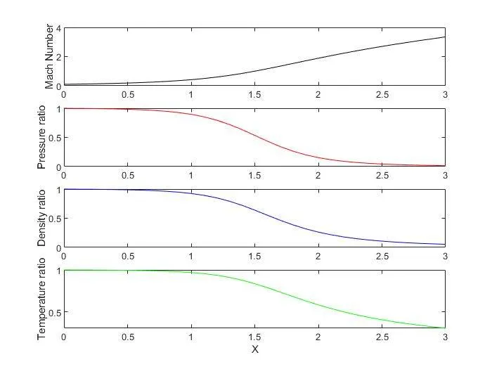
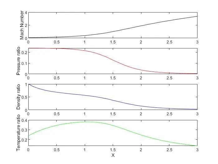
1.Qualitative aspects of quasi-one-dimensional nozzle flow:

The changes occurs in Mach number, pressure ratio, density ratio and temperature ratio with respect to the value of x is analysed.

Non conservative method:

Conservative method:

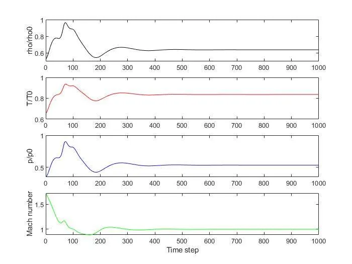
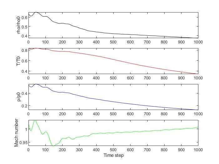
2. Timewise variations of the density, temperature, pressure, and Mach number at the nozzle throat:

The variation of density, temperature, pressure and mach number with respect to the time step at the throat region of the nozzle is analysed.

Non conservative method:

Conservative method:

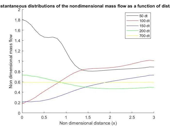
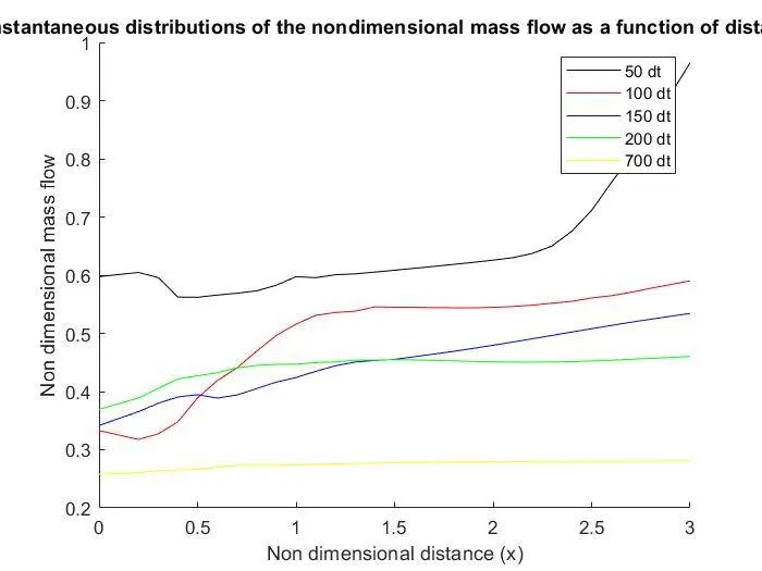
3. Instantaneous distributions of the nondimensional mass flow as a function of distance:

The mass flow rate at various distance values at the throat region with respect to the nun dimensional distance is analysed.

Non conservative method:

Conservative method:

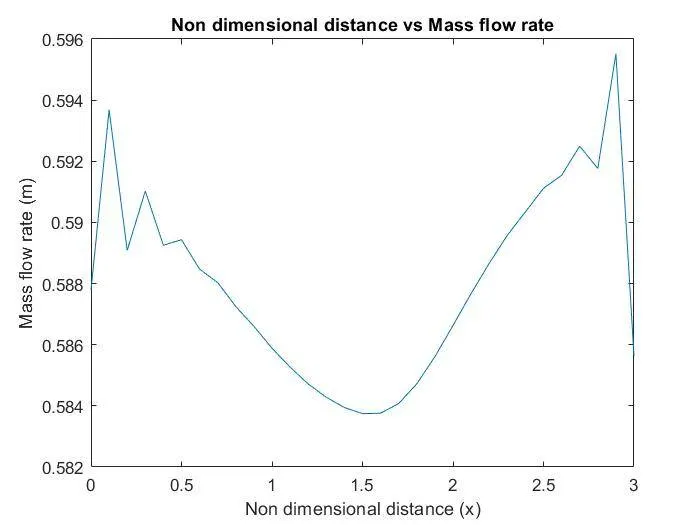
Comparison of Normalized mass flow rate distributions:

The normalized mass flow rate at two different methods with respect to non dimensional distance is analysed.

1. Non conservative method:

In non conservative method, the mass flow rate initially rises to maximum and then drops down and it reaches the maximum value at the end. It depicts that the mass is minimum at the throat and maximum at both the convergent and divergent section.

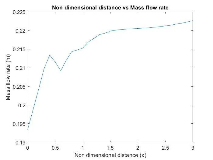
2. Conservative method:

For the conservative method the mass flow rate gradually increases and exhibit some neck drop at middle and then it increases gradually.

Grid dependency test:

The changes in various parameters under different grid size is observed. The grid size is increased by 31,61 and 91 and the respective changes were visualized. Here the changes occurs in density, temperature and mach number by varying the grid size is shown.

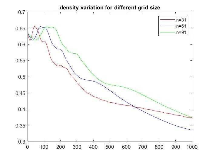
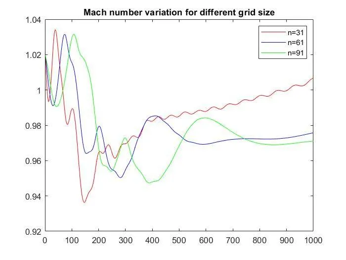
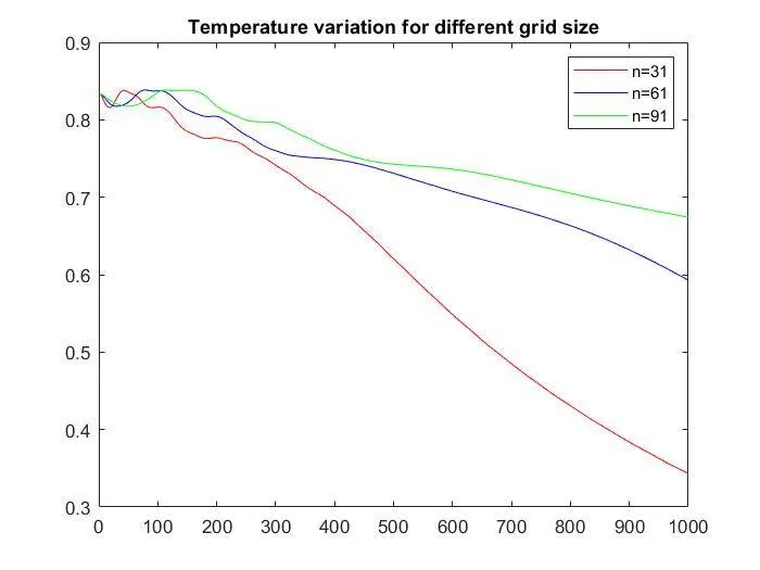
As the grid points values get increased, the accuracy of the parameters incrases. So it takes more time to get the results.

Results and discussions:

• The Mach number variation and pressure ratio are likely similar for both conservative and non conservative methods.
• The density ratio maintains a constant value till the neck region and then it gradually decreases in non conservative method. For the conservative method, it decreases gradually from the inlet of the nozzle itself.
• The temperature ratio decreases from the maximum value in the non conservative part. But in conservative method, it starts from the lowest value and increases near the throat and then gradually decreases.
• The parameters at the throat region of the nozzle maintains an optimum value in the case of non conservative part, while in conservative part it gradually decreases.
• The mass flow rate at various distance corresponds to the x value is analysed. The straight line at 700dt is the steady state result. This one is obtained with a mass flow rate of 0.6 for non conservative method and nearly 0.25 for conservative part.
• The normalised mass flow rate was also analysed.
• The grid dependency test was done. The values or parameters not differes much by increasing the grid size. The three grid sizes 31,61 and 91 gives converged results with good accuracy.
• The time taken for getting the converged results are not differ much for the three grid size values. So n=31 is enough to get the converged results.

Finally, by analysing the various factors conservative method will be the right method for solving the problems using macormack method. It give accurate or converged results without droping the mass flow rate. It maintains an optimum mass flow rate throughout the analysis.

Conclusion:

Thus, the 1D supersonic nozzle flow simulation is made using MATLAB.

Reference:

COMPUTATIONAL FLUID DYNAMICS
The Basics with Applications

by John D. Anderson, Jr.
Department of Aerospace Engineering
University of Maryland

Keywords: CFD, Quasi, Supersonic, Macormack method, conservative, non conservative, MATLAB, Density, Boundary condition.