Roof Crashworthiness analysis of Dodge Neon Model using Radioss and HyperCrash

AIM

To carry out a Quasi-static Roof crush analysis on a Neon Dodge model using Hypermesh/Hypercrash (pre-processing) and RADIOSS (solver)

OBJECTIVE

• Open the Neon Dodge model and the impactor model is to be placed in such a manner to crush the roof of the car model.
• Plot force vs. displacement. Check that the FMVSS 216 target load of 47,000 N (= 3 * GVW) has been met.
• Plot the energy vs. time curves

Model Setup and Execution

We need to open the car model in the Hypermesh atmosphere by importing the starter neon_roof_0000.rad file. After that, we need to import the FMVSS_216_ROOF_IMPACTOR_coarse_0000.rad which is one of the standard impactors used for Roof crush analysis.

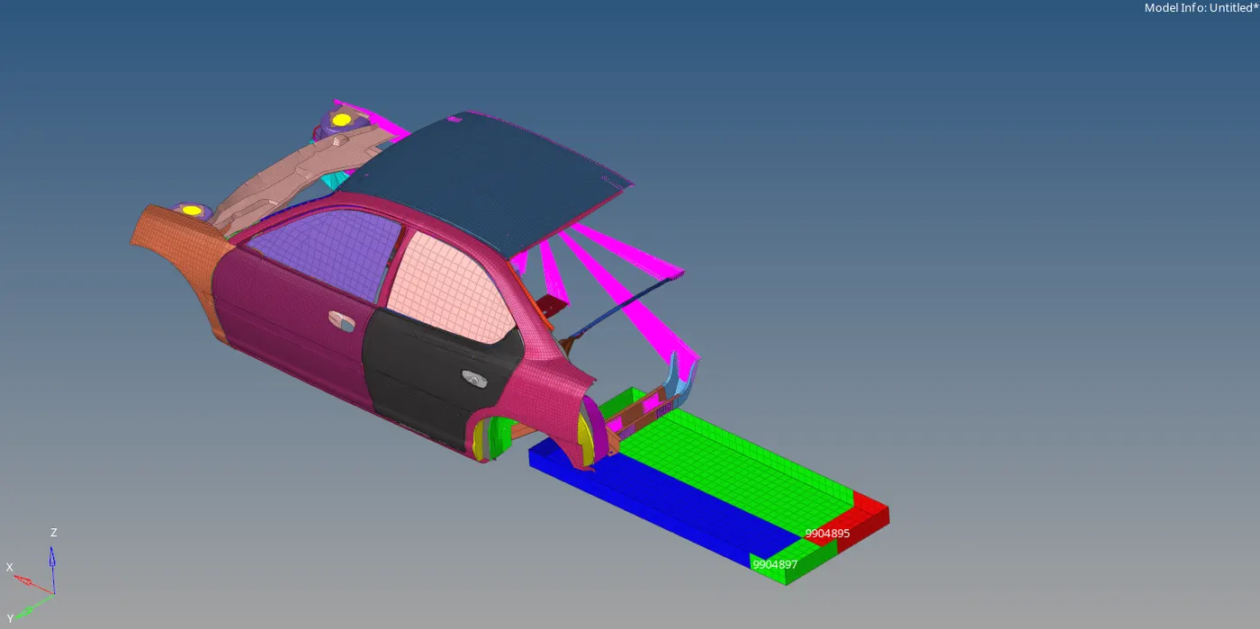
Fig: Files imported view

1. After importing both, we need to orient the impactor in a way that it is in an inclined manner position above the A-pillar (but starting impact near to the B-pillar) frame. The positioning reference is done by the following steps,

1. A 180° rotation about the global z-axis
2. A 5° rotation about the axis through axis AB
3. A 25° rotation about the axis through axis AC
4. A translation to put point A at global ( -3250.00, 584.822, 1343.06)

The step-1 is executed as shown below by using the Tools > Rotate > Component > z-axis > 180deg

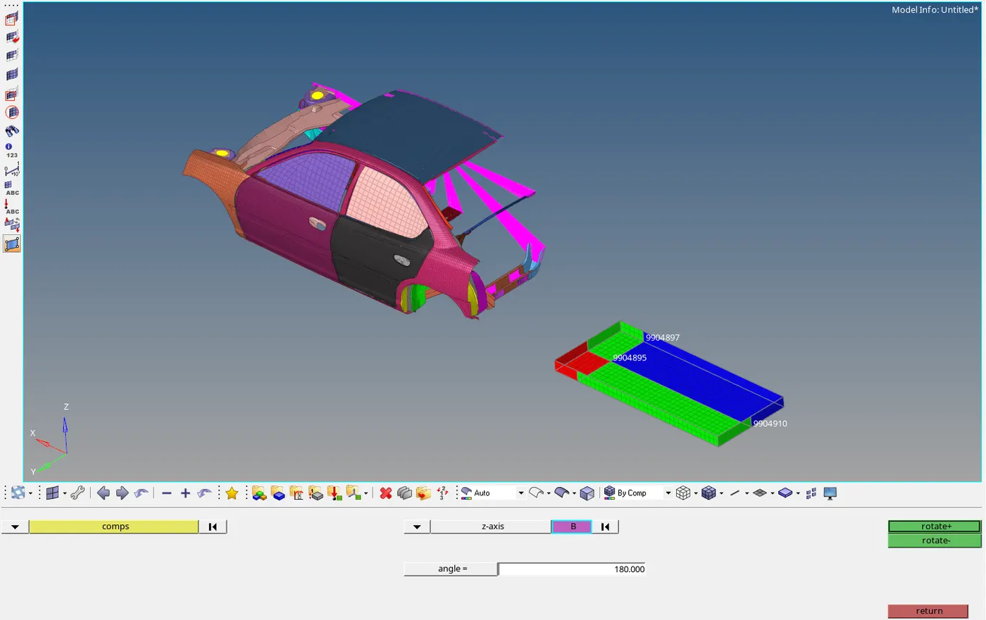
Fig: Image represents the rotation made in the z-direction

The step-2 is executed as shown below by using the Tools > Rotate > Component > y-axis > 5 deg

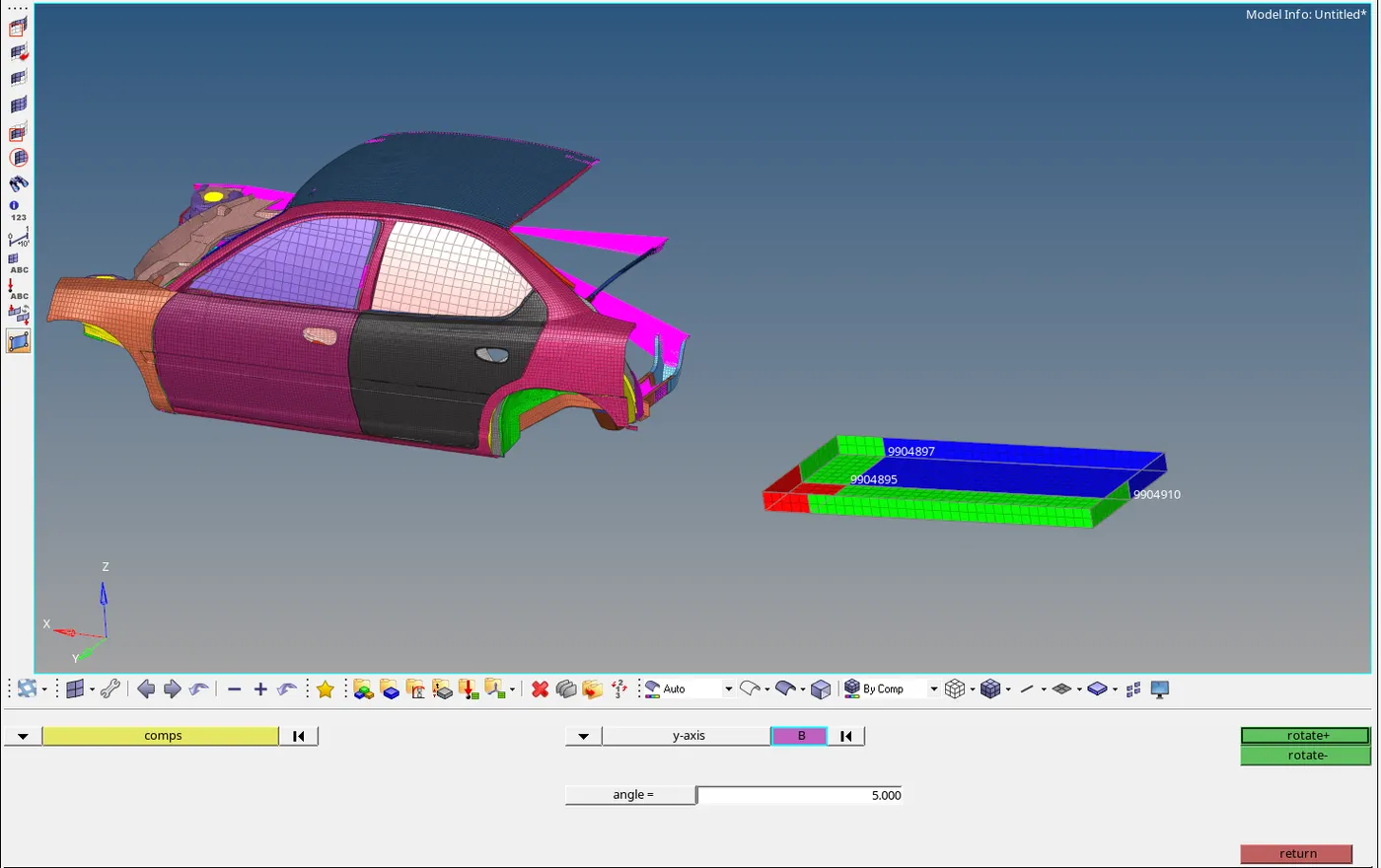
Fig: Image represents the rotation made in the y-direction

The step-3 is executed as shown below by using the Tools > Rotate > Component > x-axis > 25 deg

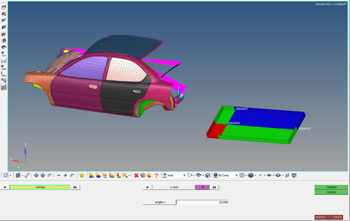
Fig: Image represents the rotation made in the x-direction

Finally, in step-4 the translation is made to put point A at global ( -3250.00, 584.822, 1343.06) and some movement is done in the x-axis so as to position the impactor to a specific region as mentioned in the image below. The final coordinate movement in A point is given by ( -2450.00, 584.822, 1343.06).

Tools > Translate > Component > select the axis > magnitude > translate+ / translate-

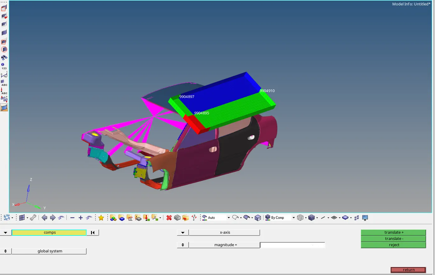
Fig: Final view of Impactor placing with roof

Here we need to save this arrange the position of the impactor with the Neon Dodge model as a single rad file for future usage and we saved as roof crash_final_0000.rad. For further setup, we can use the Hypercrash atmosphere for our convenience and later can be imported for the solving purpose.

2. Create an appropriate interface, friction 0.2, and recommended parameters.

Here we need to create a type-7 interface between the roof and the impactor since it is essential because the roof and impactor will interact when the crash happens otherwise the impactor will pass through the car roof that causes an intersection. The Impactor is taken as Master since it is coarse meshed and it is much more rigid, while the entire car parts are defined as Slave since we need to study the deformation in the car component.

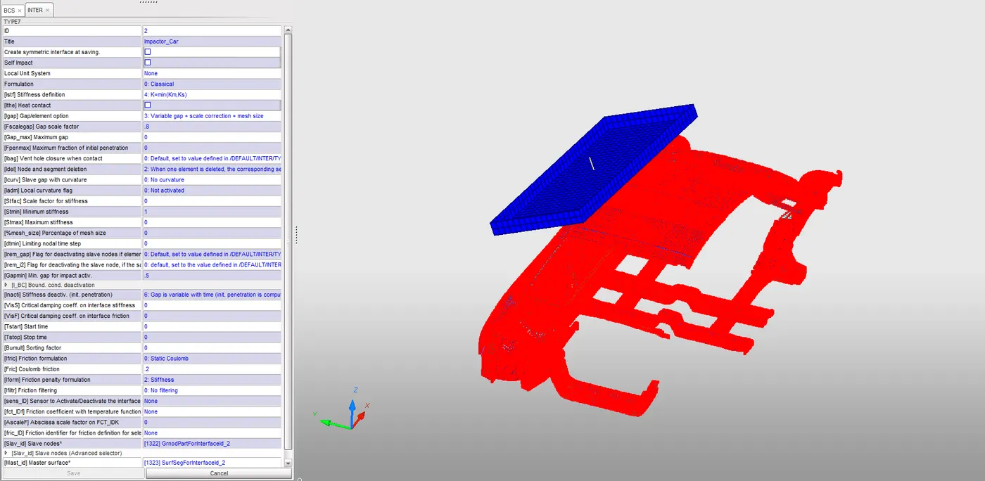
Fig: Contact defined between car and the impactor (Type-7)

Also, a Self-contact is created in order to prevent the penetrating of nodes into the elements while the deformation caused by the impact. Type 7 contact is created between them and the self-contact is defined with their commended parameters like Igap =3, Inacti =6, Istiff =4, Gapmin =0.5, Idel =2, Iform =2.

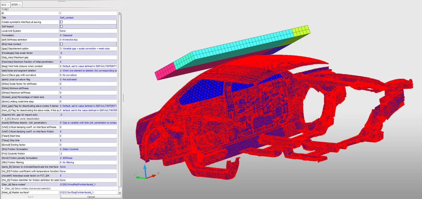
Fig: Self-contact (Type-7)

3. Make sure of no penetrations, intersection, and Proper connectivity between parts(ie, No free parts)

To check for the intersections and penetrations of the parts using tree-selection can be done by selecting Quality > Check Intersections of Tree Selection

Before moving to the next step we will make sure there are no intersection or penetration of elements. If any, fix them by using the tools provided in Hyper-crash / Hyper-Works, since there was no penetration or intersection during the check we can proceed further.

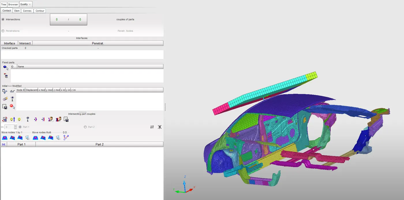
Fig: Intersection check

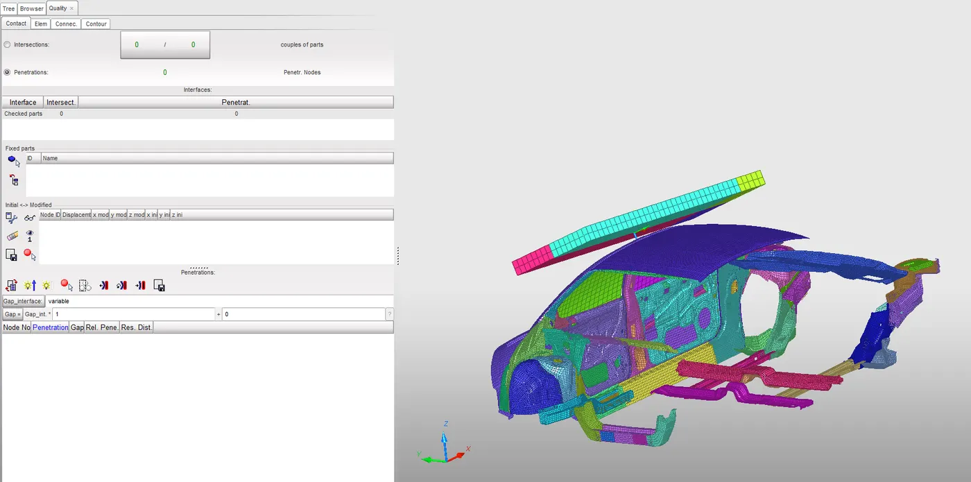
Fig: Penetration check

Note: Now we need to check for the connectivity of the parts

To check for the connectivity of the parts using tree-selection can be done by selecting Quality > Check Connectivity of Tree Selection. It will show a list of free parts and joints. These are the parts and joints which are not connected to any of any parts. To compare with the full model and check whether the part where the joints are connected to are presented in the surrogate model, If not then delete those joints. And if some parts are free then connect it to its respective component using some sort of simple springs. Always make the model a single connected one or otherwise run issues will occur.

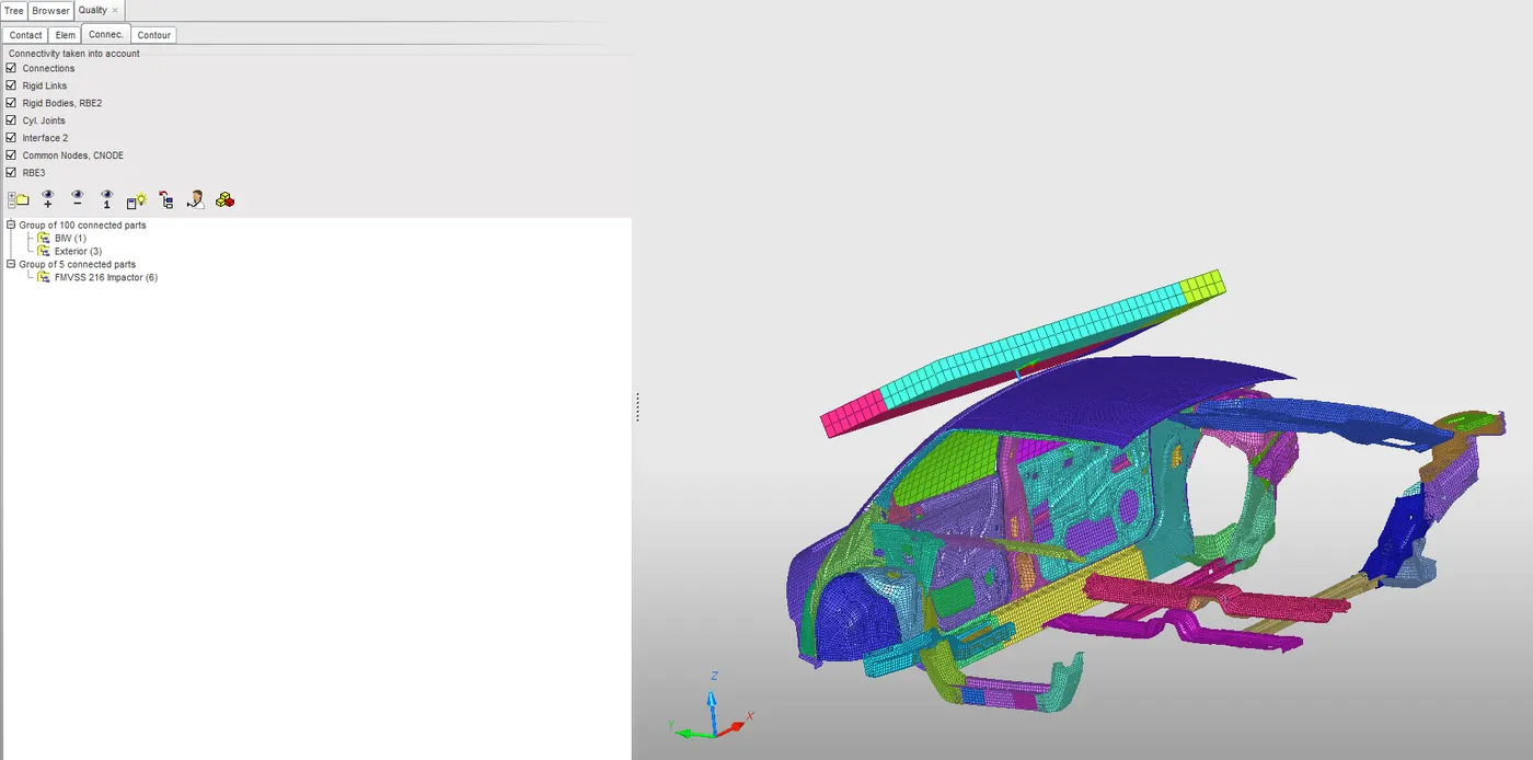
Fig: Connectivity check

4. Boundary condition defined in the model

BCS of the suspension shock tower: Here we need to lock the suspension shock towers on the z-axis. For that, we first create the rigid bodies to connect the suspension nodes to a single master node this is done for all the three suspensions that exist in the model. Then we apply the Boundary condition for the 3 master nodes of the suspension. While creating the BCS the Z-axis should be checked to arrest the degree of freedom in that direction.

BCS of the Impactor Spring: Here we need to move only one node of the impactor spring ie, one end on the rigid connection of the impactor. For that, we need to arrest the D.O.F of the free node of spring in all the 6 d.o.f.

BCS of the Impactor Rigid Body: Then we need to arrest all D.O.F except the z-direction for the Impactor Rigid body. While creating this we should also create a moving SKEW to represent the normal to the face of the impactor. This normal should be the z-axis of the moving skew just created.

BCS of the right end rigid connection: Here we need to arrest the D.O.F of the master node of a rigid element connection in all the 6 d.o.f.

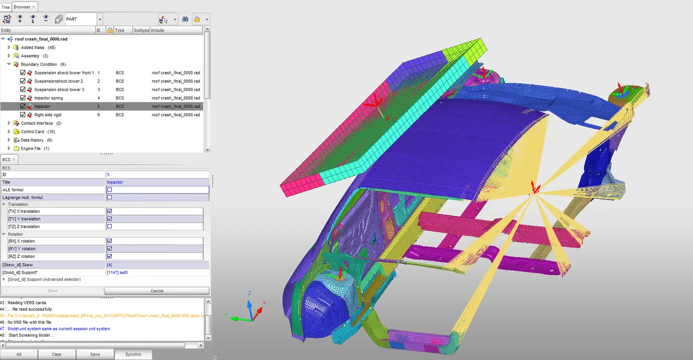
Fig: Boundary condition defined for the model (element-wise view)

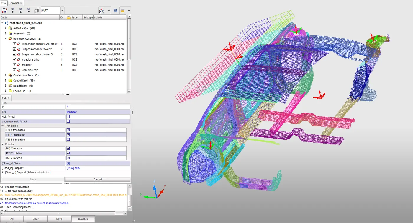
Fig: Boundary condition defined for the model (wire-frame view)

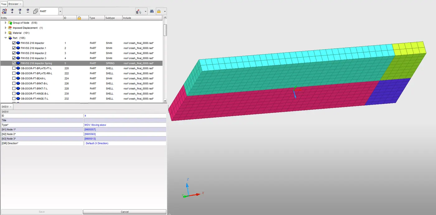
Fig: Moving Skew created for the Impactor

5. Set up Imposed Displacement

Here we need to define the Imposed displacement for the impactor. Along with that, we need to define the function with the displacement as 0mm at 0mm/ms velocity to 200mm displacement at 200 ms time. If the direction of application of the velocity is not in the downwards direction put the scale factor as a negative one to adjust the direction.

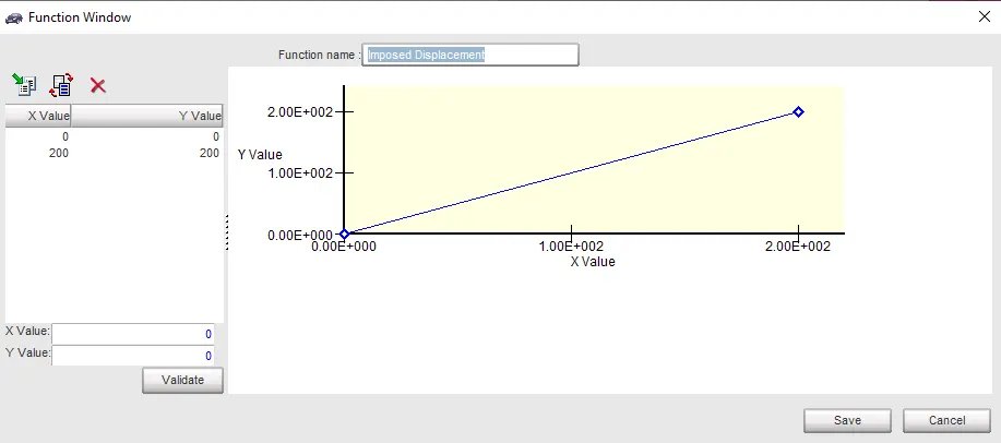
Fig: Function card defined for Imposed displacement

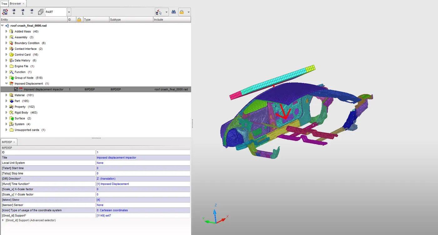
Fig 9 Imposed displacement for the Impactor

6. Output TH request and Engine cards

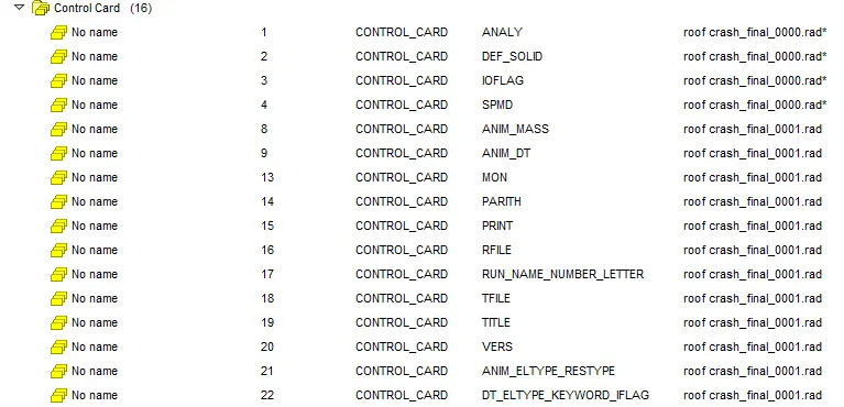
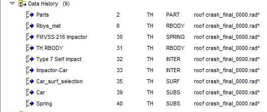
Fig: Shows the defined control cards and requested Time History output

In the control cards check the cards such as ANALY card, /DEF_SOLID card, /IOFLAG card, SPMD card, and /TITLE card. Then in the engine Control cards Check the ANIM_DT card and input 5 ms in Frequency to obtain the animations every 5 ms. Then Check ANIM_NODA to get the animation of the mass variation. To save the data in the time history check TFILE card and input the frequency to input the data in time history as 0.1 ms. To get animations of the Von Mises strain, Plastic strain, energy, Hourglass energies we need to check the ANIM_ELTYPE_RESTYPE Card.

To get the displacement and velocity which are vector quantities we need to check ANIM_VECT Card. Check the Run Card and input the termination type as 200ms. This much time is given since the quasi-static analysis done using an explicit solver need to run for this much time so that the inertia factor will be insignificant. If inertia is dominant then the equilibrium in every time increment is not possible. So to keep the model in every time increment in equilibrium we need to run the simulation for 200ms. And Turn ON the /PARITH Control Card as well.

7. Run the model checker and debug the errors and warnings.

Finally before generating the radioss simulation and file we need to do the final check i.e. model check. On running the model check we see that it showed a few errors and warnings so we need to check and fix them. The error can be due to unused group nodes, shells, surfaces, etc. It can be also due to the incompatible kinematic condition or wrong definition of rigid connection, etc. By working on the errors, finally, we got the debugging correct and manage to fix all errors. Here the warning will not affect the simulation of our file and this arises due to the better definition of the cards for the proper simulation.

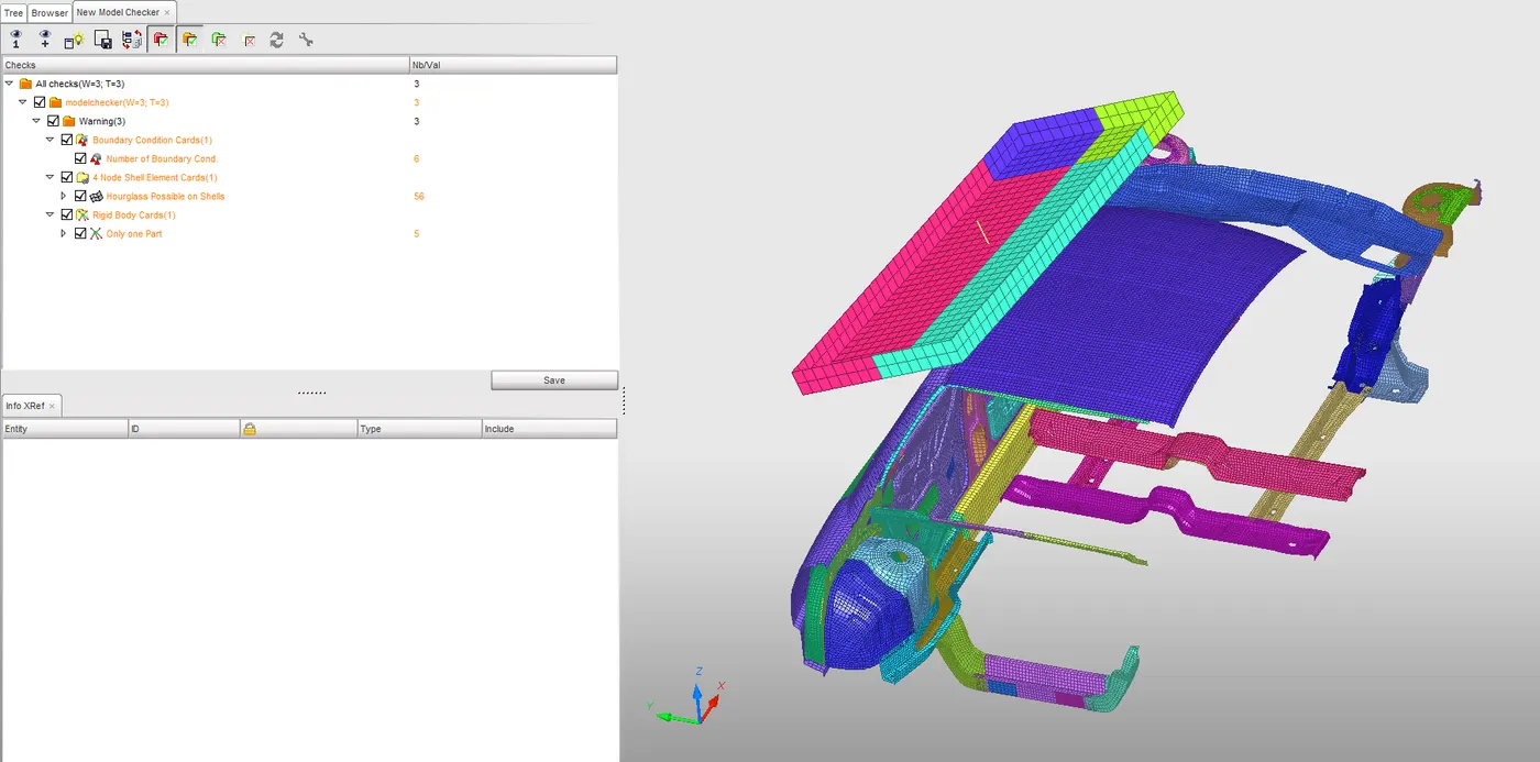
Fig: Debug the errors

Finally, we can export the file to Radioss and then open it via hypermesh and run the analysis using 4 core of CPU by input the -nt 4. After the analysis, we need to check the energy error and mass error in the simulation.

POST PROCESSING

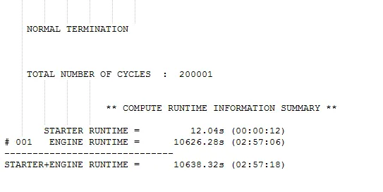
On opening the _0001.out file, we can see the energy error to be -17.9% and mass error to be 0.04673 which is acceptable and can consider an as a good model with total no. of the cycle as 200001 with time duration of 2:57:18 or 10638.32 sec. Since here the energy error values go up to -17.9% which is acceptable as energy error-values are acceptable up to 20 % and the mass error is also below 5%. So the simulation results may be acceptable.

Results

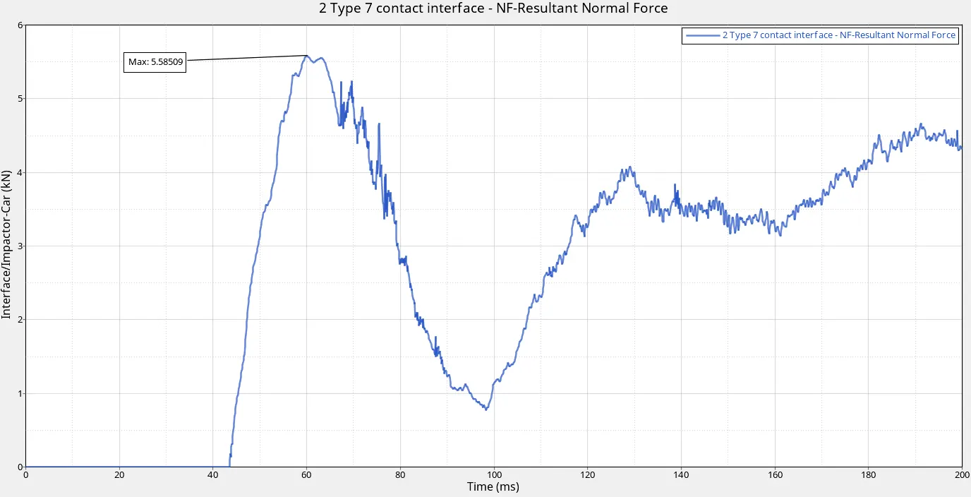
Fig: Contact interface between Impactor and Car

The force experienced by the interface between car and impactor case is shown in the graph above and the case with the self contact force will be higher than the above-published value.

To plot Force vs Displacement: However, the HyperGraph 2D plots all the parameters vs time and hence we are going to cross plot Force vs time and Displacement vs time. The Displacement vs time is plotted for a single node on the impactor which is a linear curve and the force vs time is plotted for the contact interface between the car and the impactor. Then we use the math option in the menu bar, select two curves, and keep displacement vs time in the x-axis and total resultant force vs time in the y-axis. This cross plots both the curves. The maximum value of force obtained from the plot is 5.69kN

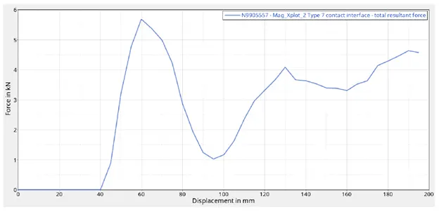Fig: Force vs Displacement curves

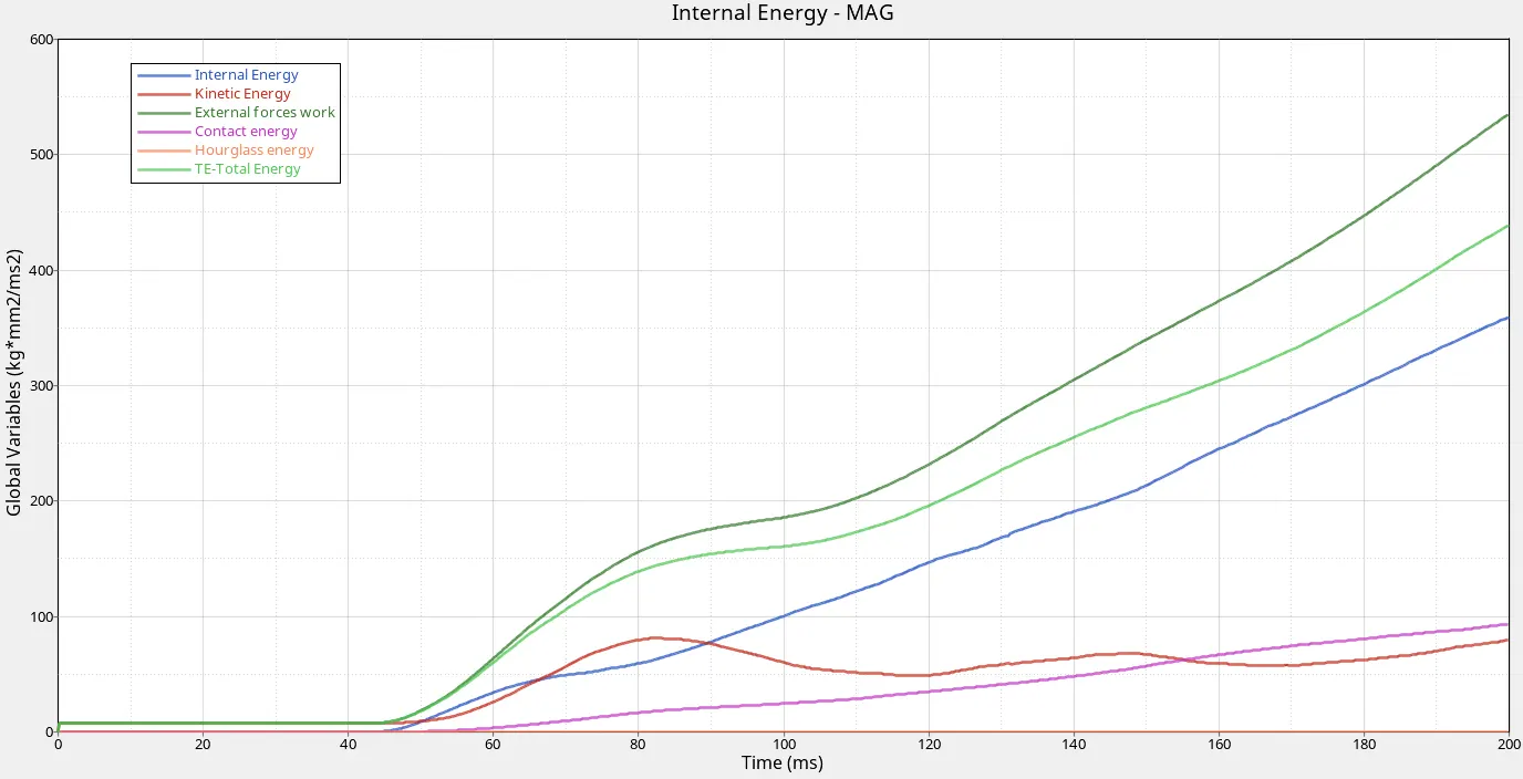
Fig: Energy Curves

The value of Internal energy is closer to 360kg*mm^2/ms^2 and the value of kinetic energy is closer to 80kg*mm^2/ms^2 which is 14% of the total energy. The reason for the lower kinetic energy is because this simulation is a quasi-static one rather than an explicit analysis (like frontal/side crash analysis) as the car is stationary and not moving. The contact energy keeps increasing gradually to a maximum value of 90kg*mm^2/ms^2 while the hourglass is very less but not zero as we would've ideally expected.

Here the mass of the vehicle is 175 kg, so weight equals 175*9.81 = 1715 N, if we consider this weight as the Gross Vehicle Weight(GVW) then 3 x GVW equals 5150.25 N ie 5.15 kN. The resistant force of roof crush, which is the peak force in the force-displacement relationship of the impactor, equals 5.69 kN, where the unloaded vehicle’s weight, W = 1715N. The maximum value of force obtained from the plot is 5.69kN which is closer to the expected value of 5.15kN which means the FMVSS crash standards are met by our model.

CONCLUSION

We can observe that quasi-static analysis is also an important aspect of Crashworthiness analysis as it involves various considerations to be taken care of and standard procedure followed. In our case, we have taken FMVSS 216, Roof Crush Resistance for our analysis to test the strength requirements of the passenger compartment roof of passenger cars. This test will help in designing the roof so that it can withstand the load acting on it and preparing for the eventuality when something wrong happens, the passengers present inside are protected.