Road Profile Modelling by ISO

AIM: To perform classification and generation of a road profile according to ISO.

GIVEN DATA:

PSD data: https://drive.google.com/file/d/0B2S2ZJKcURAmeDNFRlMtMm5MSTQ/view

OBJECTIVE:

Using the PSD data given, determine the road quality using the ISO classification. These are your deliverables:

- Plot showing ISO classification for roads A through H (Use higher end of the range for the degree of roughness)

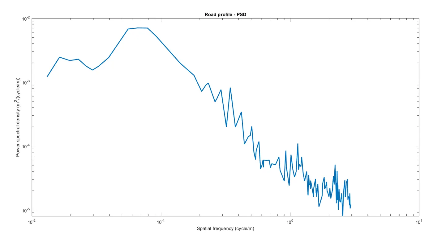
- Plot showing the PSD profile

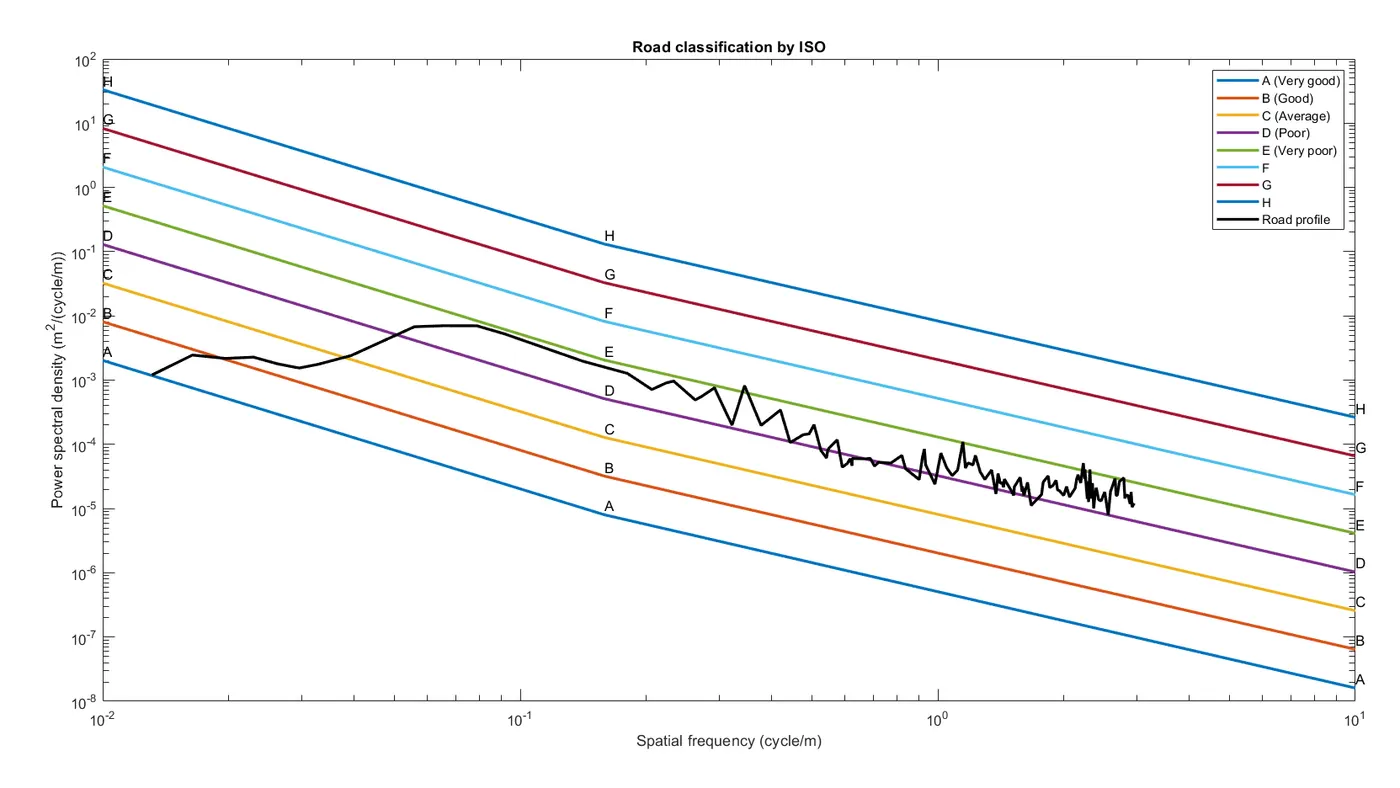
- Overlay of PSD profile on ISO classification and determination of road quality

GOVERNING EQUATION:

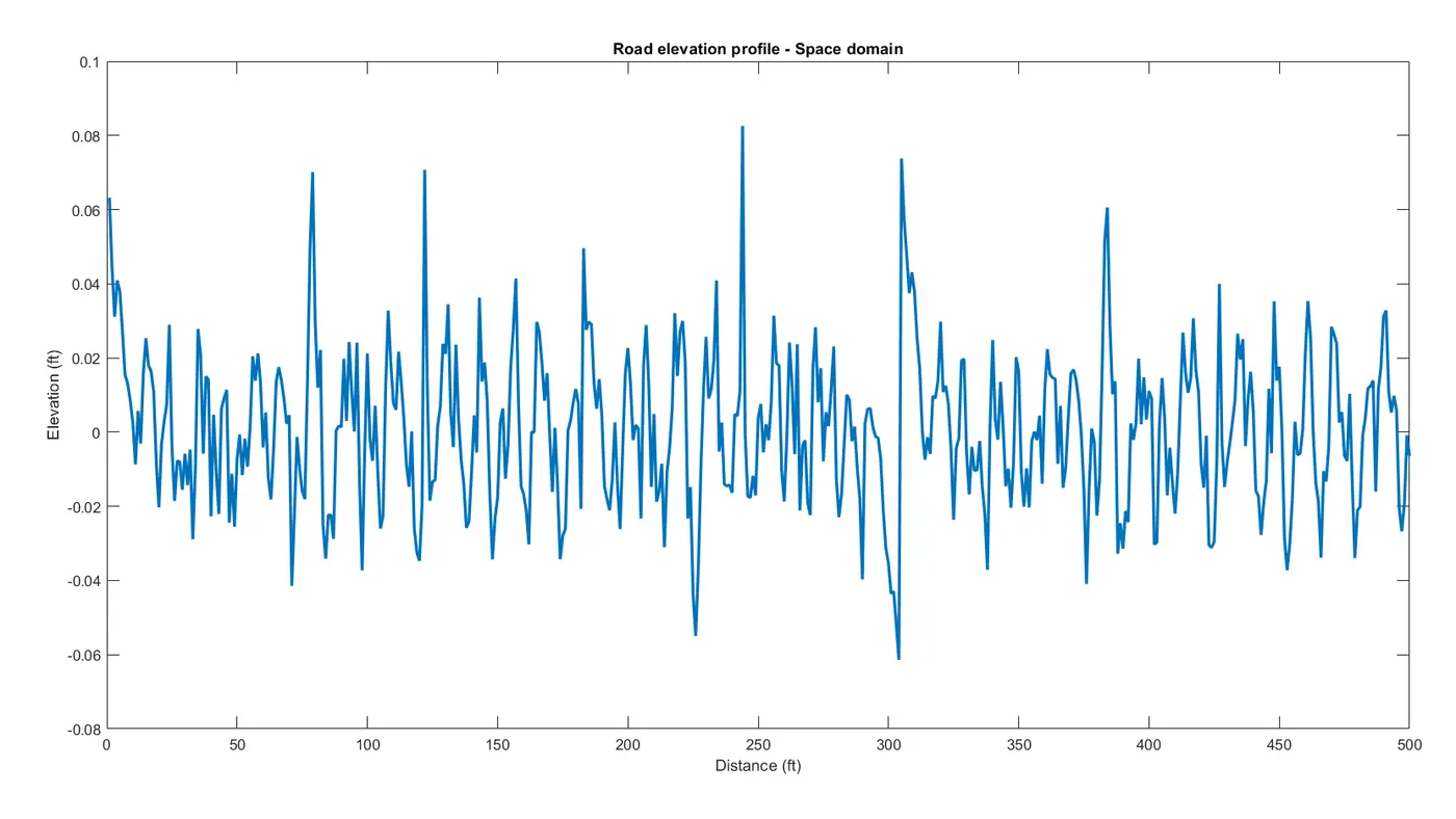
Random signal in Space domain: `z_n(x) = A_n sin((2 pi x)/(l_(wn)))`

where; `(2 pi x)/(l_(wn)) = Omega_n`

`l_(wn)` = Wavelength (m)

Random signal in Time domain: `z_n(t) = A_n sin(omega t)`

Temporal frequency (Hz or cycles/sec) = Spatial frequency (cycles/m) x Velocity (m/sec)

For `Omega < Omega_o` : `S(Omega) = S(Omega_o) (frac(Omega)(Omega_o))^-2` ... (Before the break point)

For `Omega > Omega_o` : `S(Omega) = S(Omega_o) (frac(Omega)(Omega_o))^-1.5` ... (After the break point)

where;

`S(Omega_o)` = Degree of roughness

THEORY:

Road roughness is the measure of longitudinal irregularities of road surface from the true reference plane, it plays a vital role in ride comfort and performance of the vehicle in terms of the maintenance cost, reduced speed and durability. Poor roads will increase fuel consumption, travel time and there will be more wear in spare parts of the vehicle. In other words, due to the irregular road surface, fatigue stress will act on the vehicle subsystem.

• In a random signal we are concerned with the power rather than the amplitude.
• The power spectrum can be calculated by multiplying the FFT by its complex conjugate which eliminates the phase information.
• To obtain the power spectral density (PSD), the power spectrum is divided by the frequency increment or bandwidth. It is the plot of signal power (amplitude squared) v/s frequency (spatial frequency = cycles/m).
• This ensures that the power level will not change when the frequency resolution is modified.
• PSD is a plot that has units of amplitude squared per hertz (ex: g^2/Hz for acceleration PSD)

PSD Profiles of Roads
• PSD profiles of every road section are unique.
• However, all roads show a characteristic drop in amplitude with wavenumber
• Amplitude is indicative of roughness (higher = rougher)
• The magnitude distribution in the high and low wavenumber regions determines the frequency range for vehicle vibration

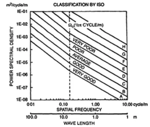
ISO Classification of road based on Road Roughness: International Organisation for Standardization gives the quality criteria as given below by plotting the graph of spatial frequency Vs Power Spectral Density. ISO classifies the roads into eight different classes, by indicating the bands of lines as shown in the figure. These bands of lines are obtained by classifying them based on the fixed PSD range. Then by overlaying the obtained PSD data with the ISO standard chart the road quality is determined. `y = mx + c` ... (Linear scale) `log y = -m log x+ log c` `log y = log x ^(-m)+ log c` `log y = log (x ^(-m) c)` `y = cx^(-m)` `S(Omega) = S(Omega_o) (Omega)^-n`

SOLUTION:

Programming Language: MATLAB

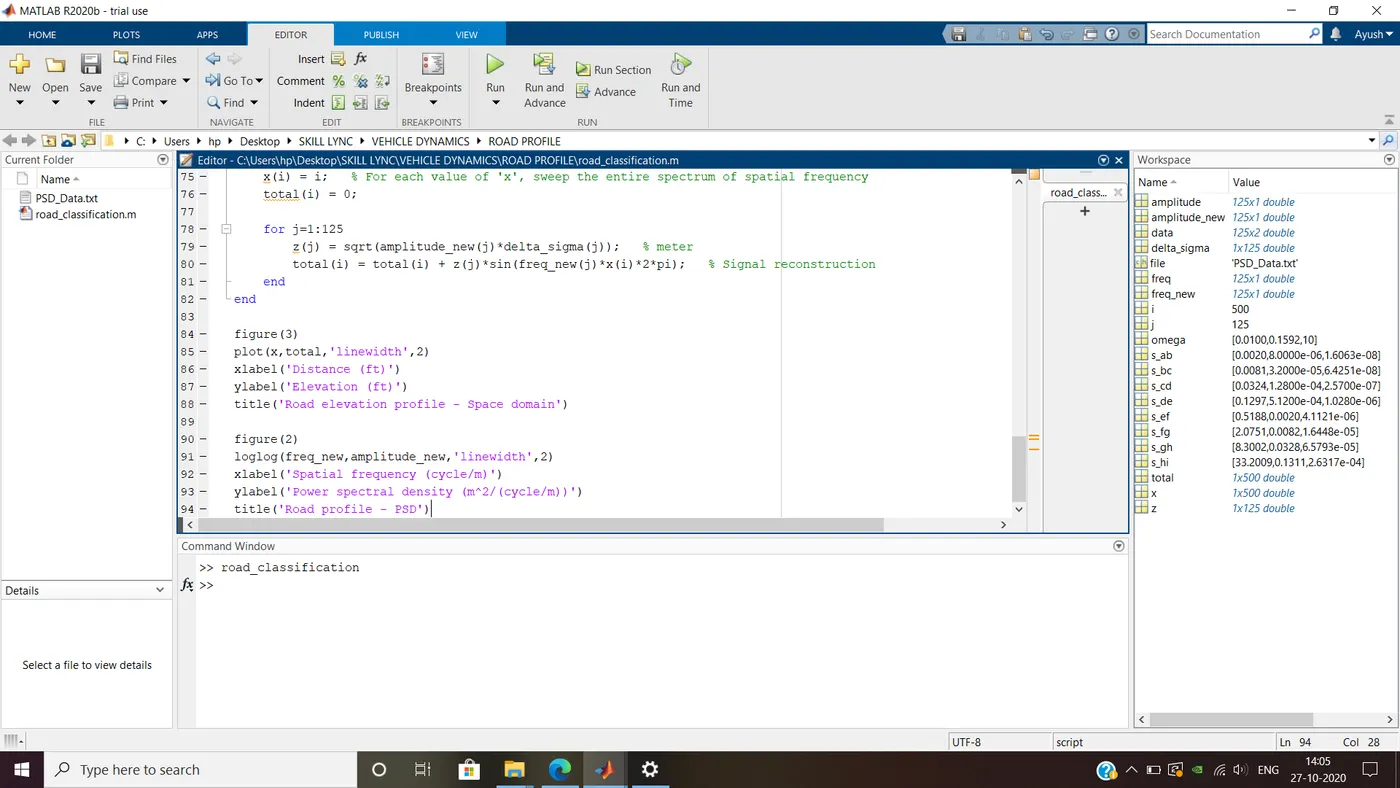
Code:

% Road roughness classification and generation

% Road data:
file = 'PSD_Data.txt';
data = importdata(file);
freq = data(:,1);        % Frequency (cycle/ft)
amplitude = data(:,2);   % Amplitude (ft^2/(rad/ft))

% End points of frequencies
omega(1) = 0.01;
omega(2) = 1/(2*pi);
omega(3) = 10;

% Road roughness class lines
s_ab(2) = 8e-6;
s_bc(2) = 32e-6;
s_cd(2) = 128e-6;
s_de(2) = 512e-6;
s_ef(2) = 2048e-6;
s_fg(2) = 8192e-6;
s_gh(2) = 32768e-6;
s_hi(2) = 131072e-6;

s_ab(1) = s_ab(2)*(omega(1)/omega(2))^-2;
s_bc(1) = s_bc(2)*(omega(1)/omega(2))^-2;
s_cd(1) = s_cd(2)*(omega(1)/omega(2))^-2;
s_de(1) = s_de(2)*(omega(1)/omega(2))^-2;
s_ef(1) = s_ef(2)*(omega(1)/omega(2))^-2;
s_fg(1) = s_fg(2)*(omega(1)/omega(2))^-2;
s_gh(1) = s_gh(2)*(omega(1)/omega(2))^-2;
s_hi(1) = s_hi(2)*(omega(1)/omega(2))^-2;

s_ab(3) = s_ab(2)*(omega(3)/omega(2))^-1.5;
s_bc(3) = s_bc(2)*(omega(3)/omega(2))^-1.5;
s_cd(3) = s_cd(2)*(omega(3)/omega(2))^-1.5;
s_de(3) = s_de(2)*(omega(3)/omega(2))^-1.5;
s_ef(3) = s_ef(2)*(omega(3)/omega(2))^-1.5;
s_fg(3) = s_fg(2)*(omega(3)/omega(2))^-1.5;
s_gh(3) = s_gh(2)*(omega(3)/omega(2))^-1.5;
s_hi(3) = s_hi(2)*(omega(3)/omega(2))^-1.5;

% Unit conversion
freq_new = freq/0.3048;   % cycle/ft to cycle/m
amplitude_new = amplitude*0.3048^3*2*pi;   % ft^3/rad to m^3/cycle


% Plot:

figure(1)
loglog(omega,s_ab,'linewidth',2); text(omega,s_ab,'A','VerticalAlignment','bottom')
hold on
loglog(omega,s_bc,'linewidth',2); text(omega,s_bc,'B','VerticalAlignment','bottom')
loglog(omega,s_cd,'linewidth',2); text(omega,s_cd,'C','VerticalAlignment','bottom')
loglog(omega,s_de,'linewidth',2); text(omega,s_de,'D','VerticalAlignment','bottom')
loglog(omega,s_ef,'linewidth',2); text(omega,s_ef,'E','VerticalAlignment','bottom')
loglog(omega,s_fg,'linewidth',2); text(omega,s_fg,'F','VerticalAlignment','bottom')
loglog(omega,s_gh,'linewidth',2); text(omega,s_gh,'G','VerticalAlignment','bottom')
loglog(omega,s_hi,'linewidth',2); text(omega,s_hi,'H','VerticalAlignment','bottom')
loglog(freq_new,amplitude_new,'color','k','linewidth',2)
xlabel('Spatial frequency (cycle/m)')
ylabel('Power spectral density (m^2/(cycle/m))')
title('Road classification by ISO')
legend('A (Very good)','B (Good)','C (Average)','D (Poor)','E (Very poor)','F','G','H','Road profile')

% Space domain profile from surface roughness
% NOTE: These two values are computed seperately to avoid the loop error as they do not have preceding or succeding values 
delta_sigma(1) = freq_new(2)-freq_new(1);
delta_sigma(125) = freq_new(125)-freq_new(124);

for i=2:124
    delta_sigma(i) = (freq_new(i+1)-freq_new(i-1))/2;
end

for i=1:500
    x(i) = i;   % For each value of 'x', sweep the entire spectrum of spatial frequency
    total(i) = 0;
    
    for j=1:125
        z(j) = sqrt(amplitude_new(j)*delta_sigma(j));   % meter
        total(i) = total(i) + z(j)*sin(freq_new(j)*x(i)*2*pi);   % Signal reconstruction
    end
end

figure(3)
plot(x,total,'linewidth',2)
xlabel('Distance (ft)')
ylabel('Elevation (ft)')
title('Road elevation profile - Space domain')

figure(2)
loglog(freq_new,amplitude_new,'linewidth',2)
xlabel('Spatial frequency (cycle/m)')
ylabel('Power spectral density (m^2/(cycle/m))')
title('Road profile - PSD')

Output:

Plot: