Rayleigh Taylor Instability Challenge

OBJECTIVE : Study of Reyleigh Tayor Instablity With the help CFD Simulation using ANSYS FLUENT Software .

INTRODUCTION :

• In multiphase flow , the dynamic variable like velocity , viscosity , density , pressure are generally describe and explain the flow of fluid under gravitational field and one of the basic example of its reyleigh taylor instability
• Reyleigh Tayor Instablity occures when there is change in density of flowing fluid specially when high density puts over lower density fluid under gravitational condition
  
  • Wen the density interface disturbes , heavy fluid with high density displaced downward with amount of volume of light fluid pushing upward due to sudden hydrostatic force
  • and with this amplitude of purturbation intially growing exponetially but after sometime its saturates and forms characteristic mashroom shape.
  • Daily life example : mashroom cloud like volcanic eruption, Nuclear explosion snd Plasma fusion reactors RT instability has also recently been discovered in the Sun's outer atmosphere.

• Models based on R.T Instability:

1. Ritchmyer-Meshkov instability :
   • The Richtmyer–Meshkov instability (RMI) occurs when two fluids of different density are impulsively accelerated. Normally this is by the passage of a shock wave.
   • The development of the instability begins with small amplitude perturbations which initially grow linearly with time. This is followed by a nonlinear regime with bubbles appearing inthe case of a light fluid penetrating a heavy fluid, and with spikes appearing in the case of a heavy fluid penetrating a light fluid. A chaotic regime eventually is reached and the two fluids mix. This instability can be considered the impulsive-acceleration limit of the R.T instability.
2. Plateau–Rayleigh instability:
   • the Plateau–Rayleigh instability, often just called the Rayleigh instability, explains why and how a falling stream of fluid breaks up into smaller packets with the same volume but less surface area.
   • It is related to the R.T instability and is part of a greater branch of fluid dynamics concerned with fluid thread breackupThis fluid instability is exploited in the design of a particular type of ink jet Technology whereby a jet of liquid is perturbed into a steady stream of Droplets.
3. Kelvin–Helmholtz instability :
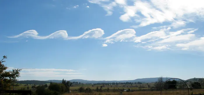
   • typically occurs when there is shered velocity in a single continous , or additionally where there is a velocity difference across the interface between two fluids. A common example is seen with wind blowing over water, the instability constant is able to manifest itself through waves on a water surface
   • 

Significance of Atwood Number :

• A dimensionless number that describes the density difference between two adjacent fluids with a common interface.
• It is used to study hydrodynamic instability in density statrified flows.

• Atwood number = ( `(rho1 - rho2)/(rho1 + rho2)`)

rho1 = Density of heavier fluid

rho2 = Density of lighter fluid

1. Atwood no. for water- Air interface = ( 999 - 1.225 ) / ( 999 + 1.225)

= 0.997

2 Atwood no. for water- Userdefined interface = ( 999 - 400 ) / ( 999 + 400)

= 0.4278

PROCEDURE :

Mainly following four parts included.

1). Pre-procesing

2). Meshing.

3). Solving .

4). Post- processing

1). Pre-procesing : It's include preparation of geometry which is being use in our simulation part .

1. After opened spaceclaim create geometry in xy plane .
2. create lower square of 20mm * 20 mm and then pull it ive name as air after moving its new component
3. create new component name as water draw upper square of same size and then pull it .

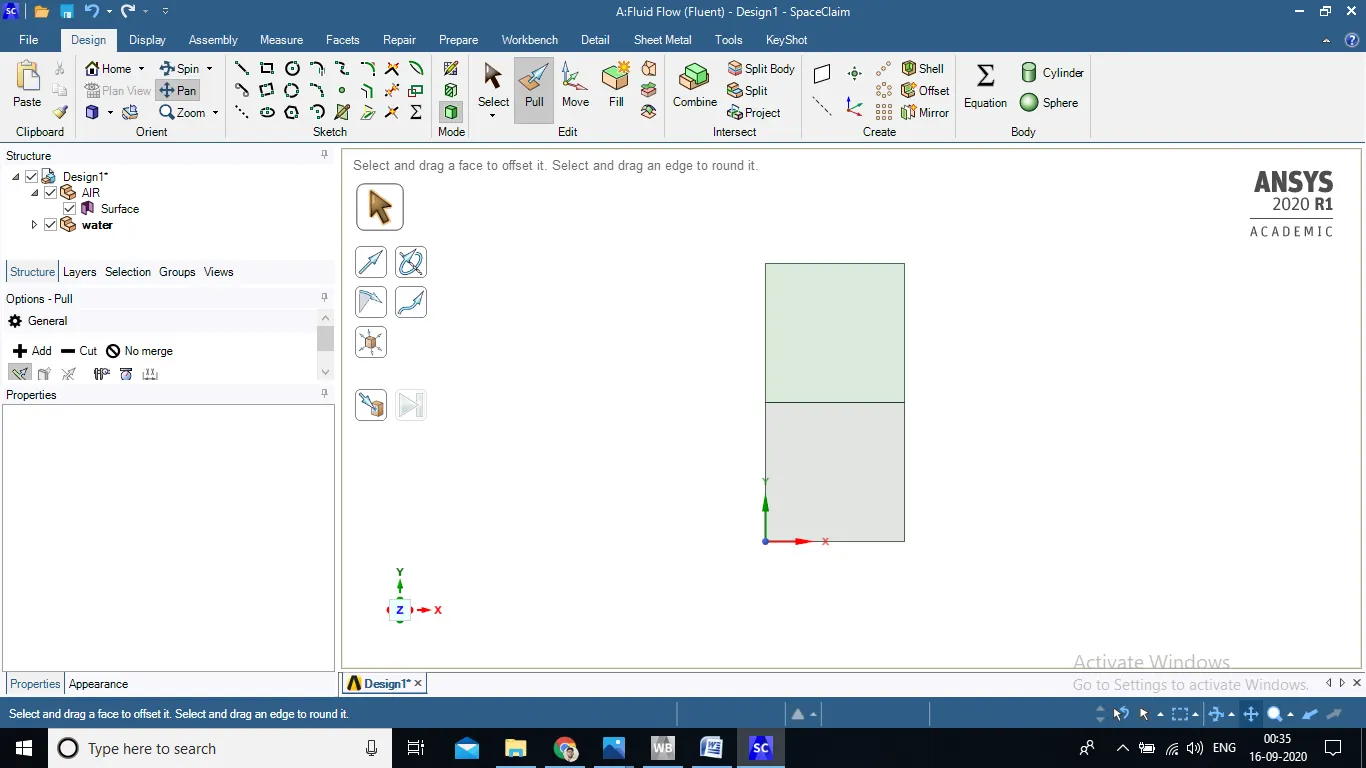
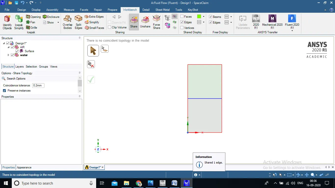
4.unable share topology and share prep after clicking on workbench

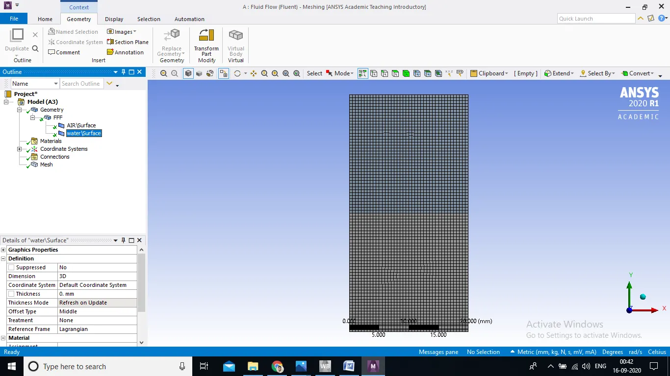
2). Meshing. :

• once geomertry created update it and open meshing and change mesh size according to case.

3). Solving

1. Unable gravity and y- direction and add gravitation constant 9.81 m/s^2
2. select transient state condition
3. add model as laminar
4. add material ( air , userdefined) by copying it from fluent database and change properties according to material

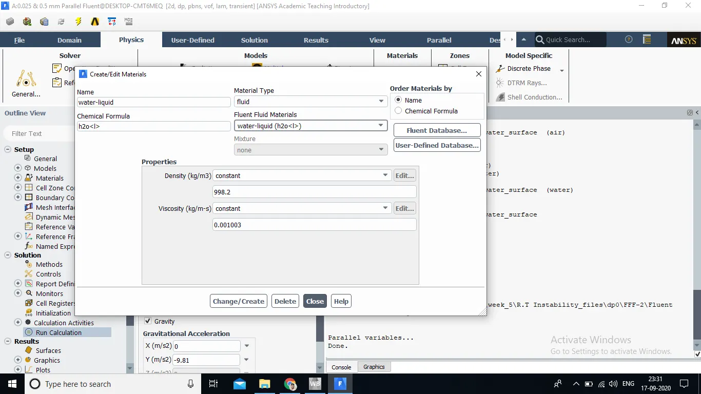
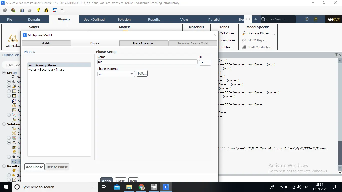
5. in multiphase model select volume of fluid method and give phase name respectively , select implicit solver.

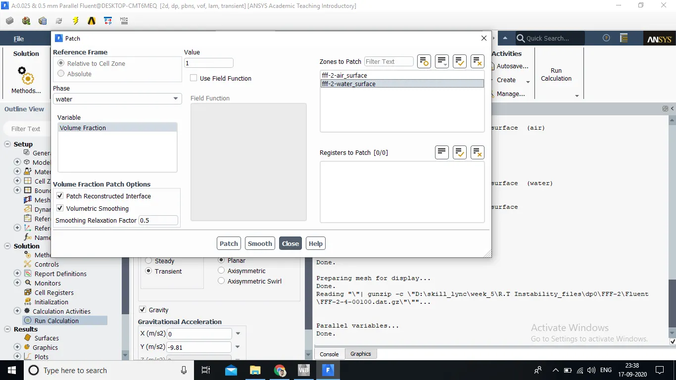
6. intialize solution (hybrid) and patch the value of water surface as 1 and air surface as 0 in volume fraction variable

4). Post- processing

DIFFERENT CASES

• CASE-1 : DIffenrent mesh size ( 0.5 mm , 0.25 mm ,0.1mm ) for same phase (air&water)
• CASE-2 : Different phase ( (air&water , Userdefined &water ) for same mesh size

• CASE -1

• Mesh size 0.5mm ( Default) for Air-water phase
  
  • No. of Nodes : 3321
  • No. of elements : 3200
  • Size of Time step : 0.025 & No. of Time- step :105

1. Residual plot

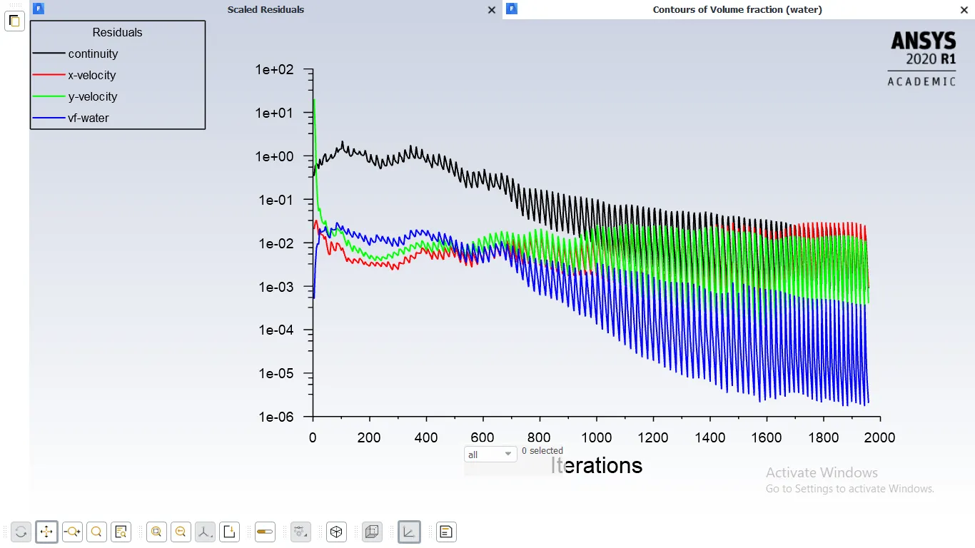
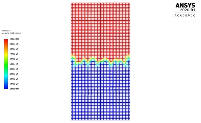
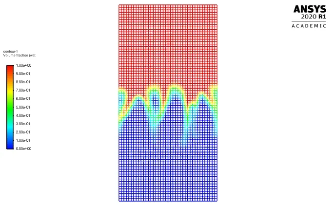
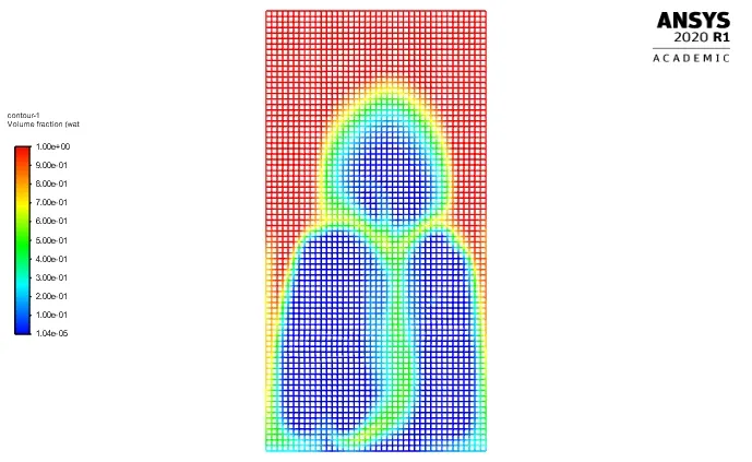
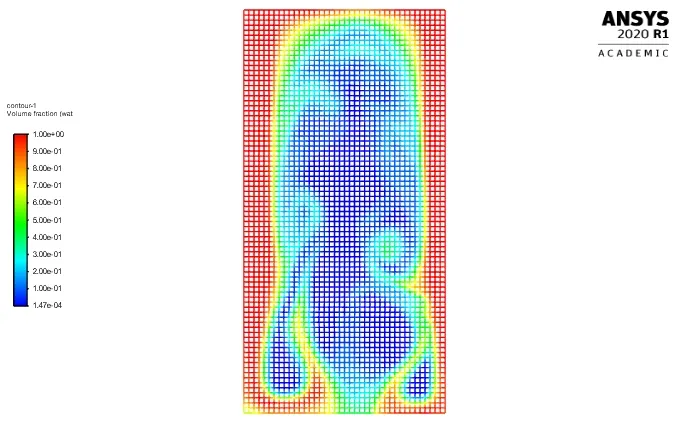
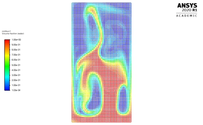
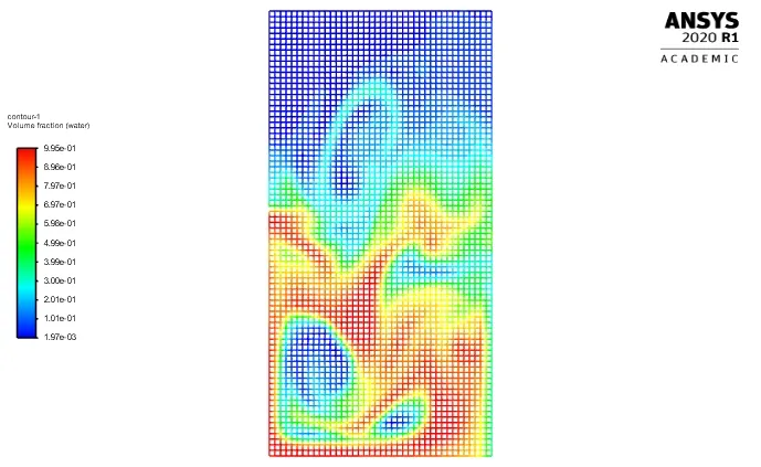
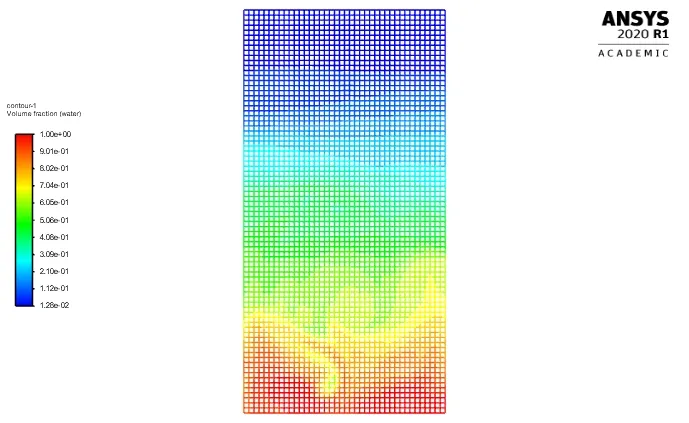
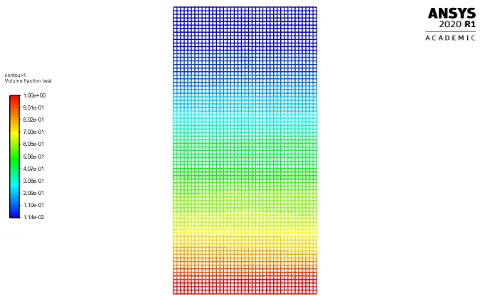
2. Contour plot of water-air volume fraction at different time ( 0.025s , 0.075s , 0.125s , 0.2s ,0.375s , 0.7s , 1.25s , 2.5s )

google drive link : https://drive.google.com/file/d/1TGIWizegFOazBJIlODXZfLqlmIiZoz_s/view?usp=drivesdk

• Mesh size 0.25mm for Air-water phase
  
  • No. of Nodes : 13041
  • No. of elements : 12800
  • Size of Time step : 0.025 & No. of Time- step :125

1. Residual plot

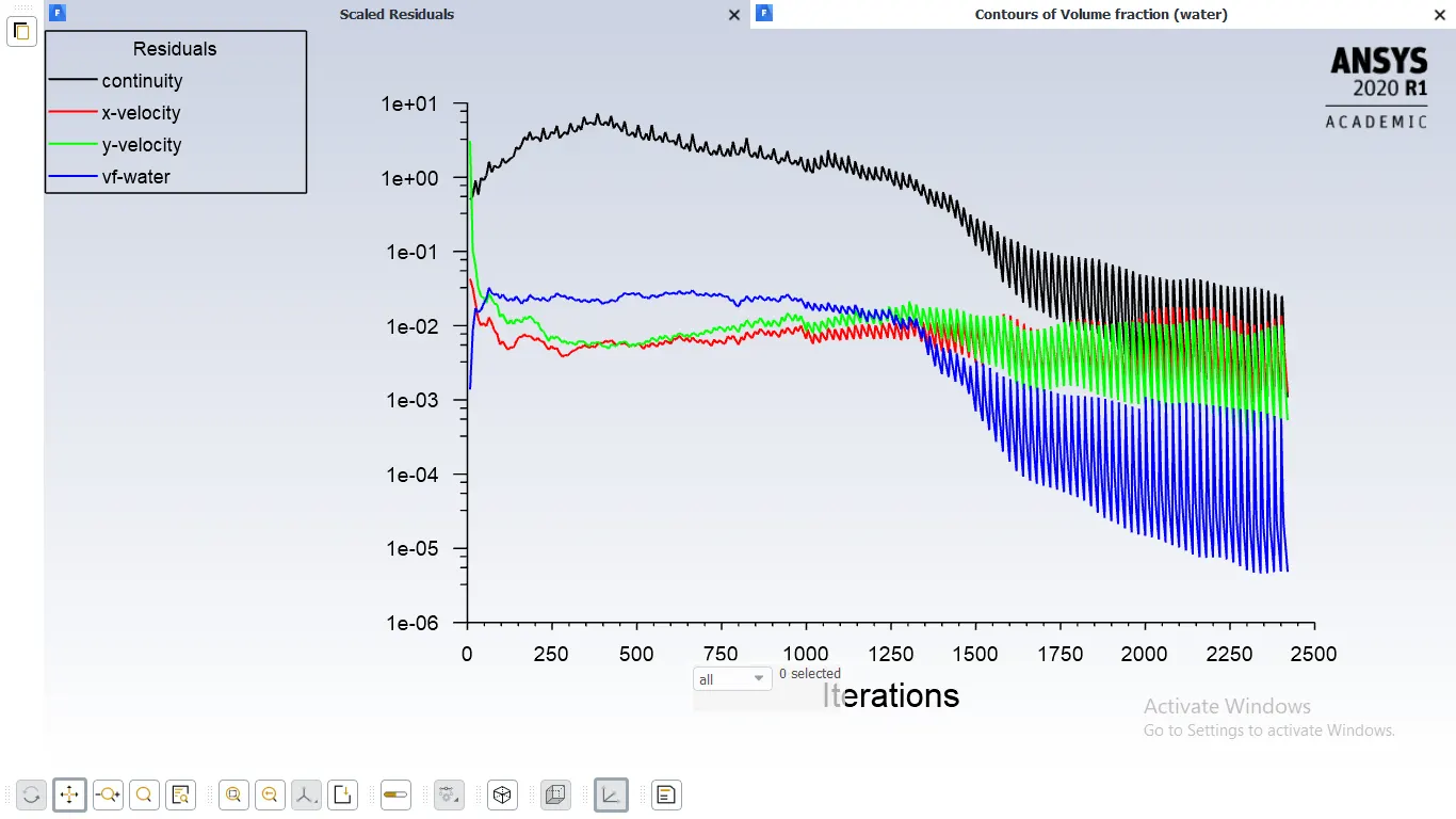
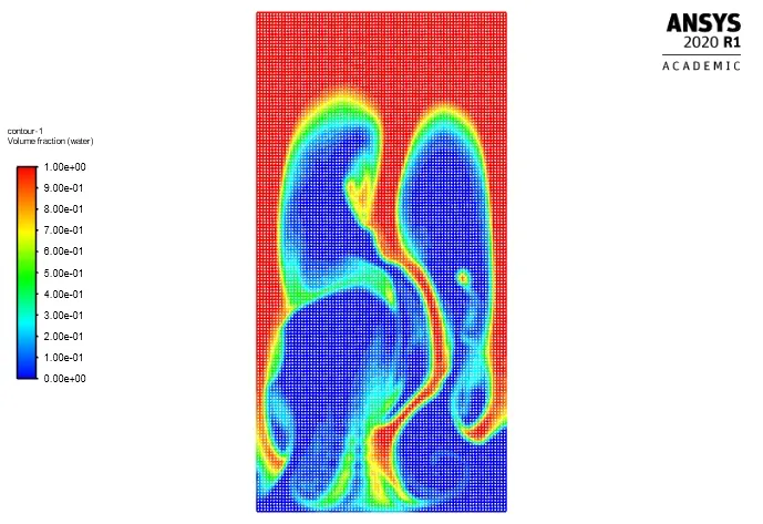
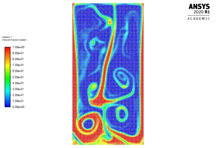
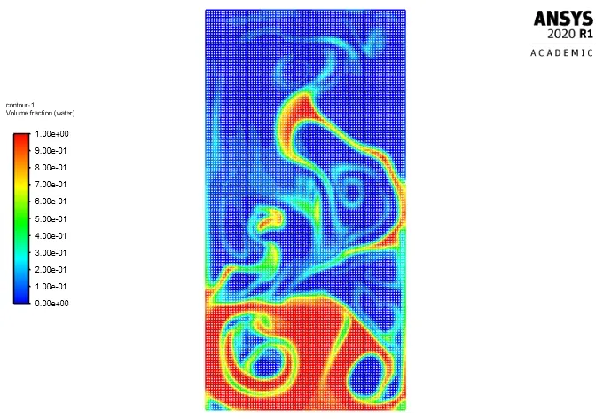
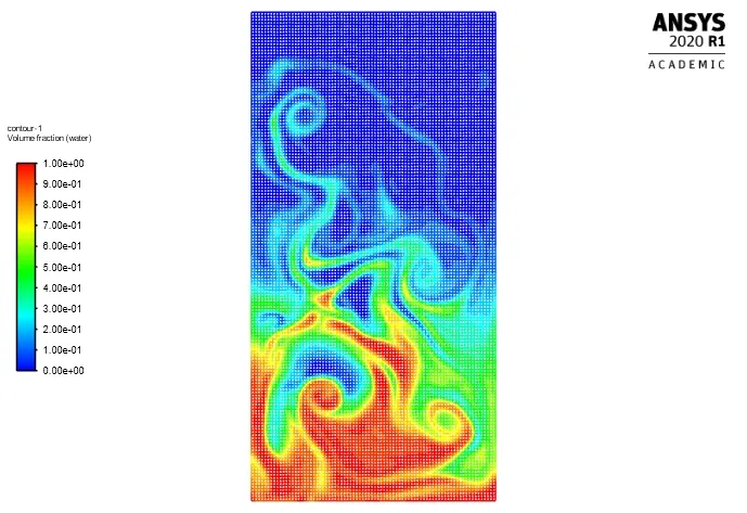
2. Contour plot of water-air volume fraction at different time ( 0.025s , 0.075s , 0.125s , 0.2s ,0.375s , 0.7s , 1.25s , 2.25s , 3s )

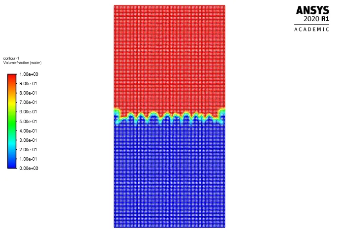
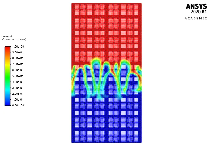
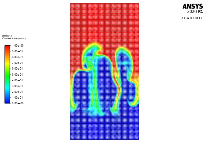
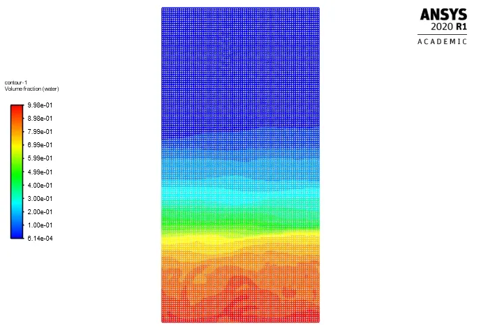
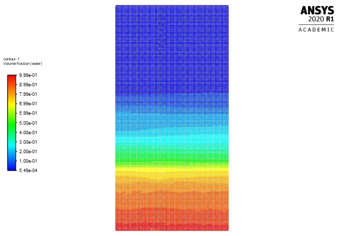
google drive link : https://drive.google.com/file/d/1AiJ6aWLokXU38owuwOjs7gAsKpQwdXvj/view?usp=drivesdk

• Mesh size 0.1mm for Air-water phase
  
  • No. of Nodes : 80601
  • No. of elements : 80000
  • Size of Time step : 0.025 & No. of Time- step :275

1. Residual plot

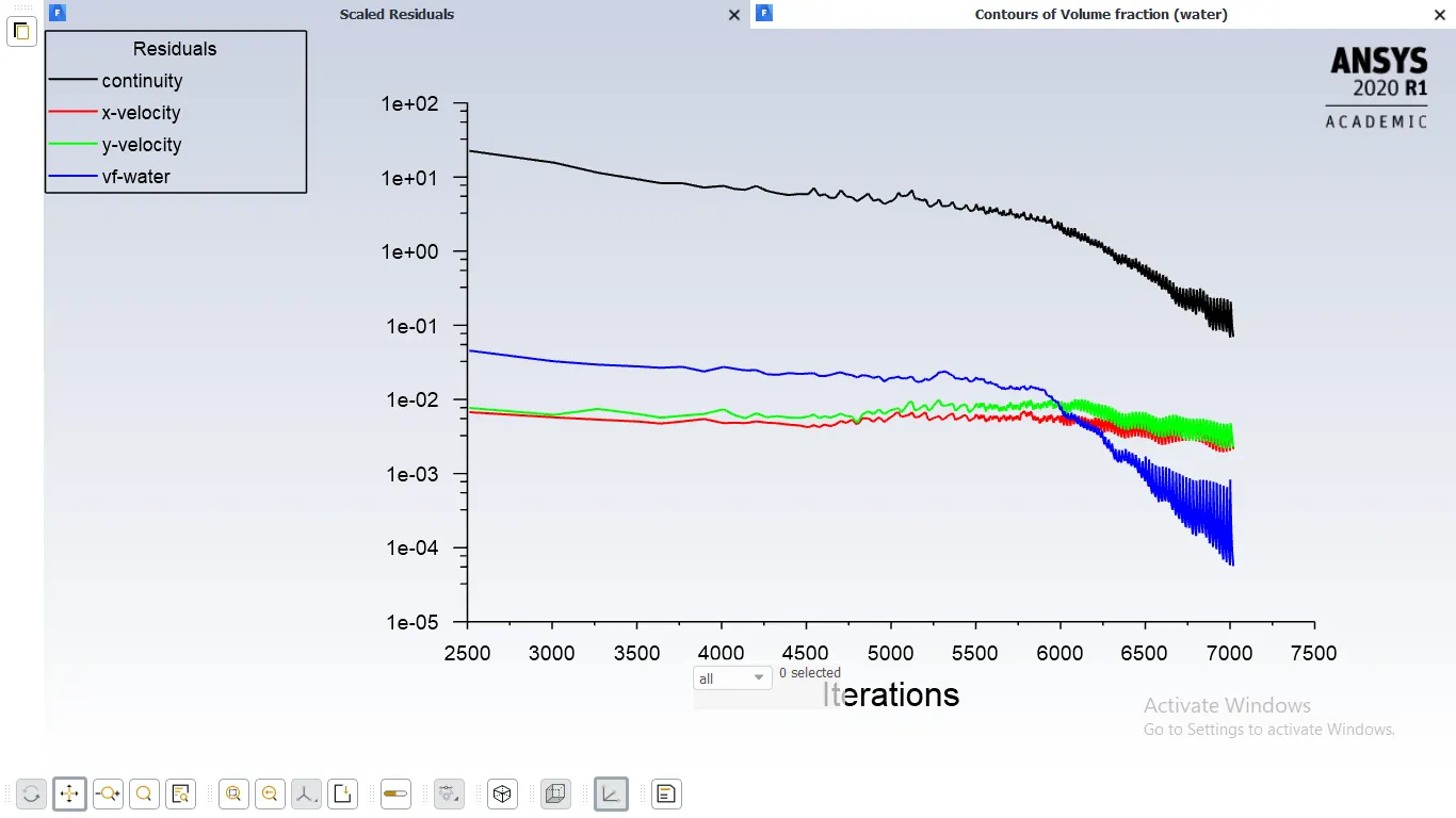
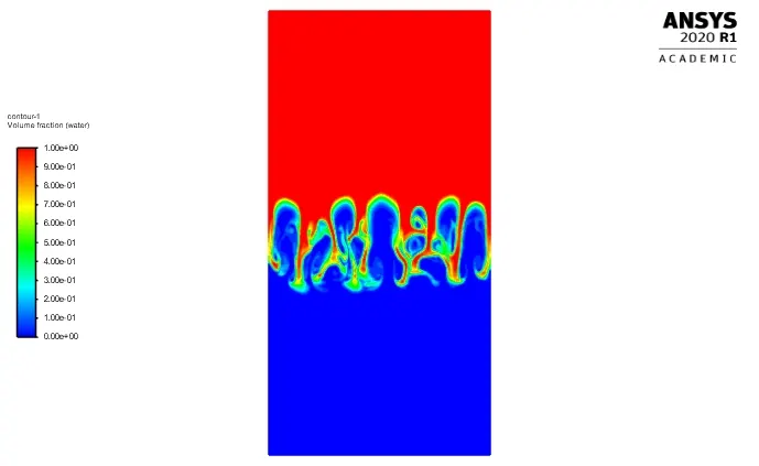
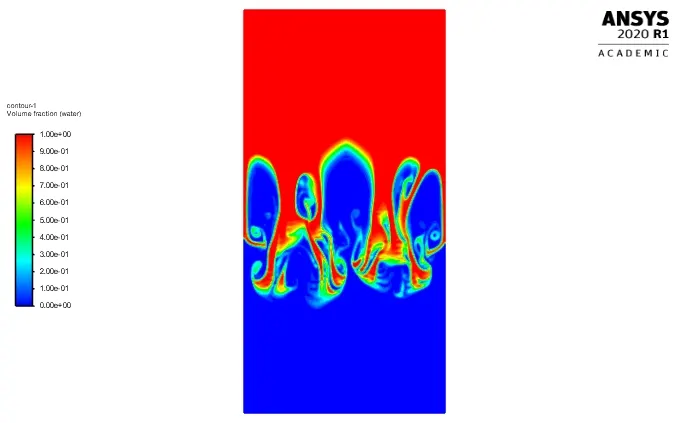
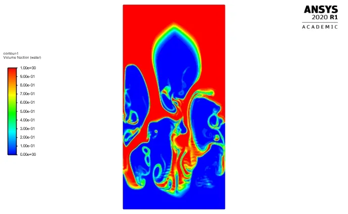
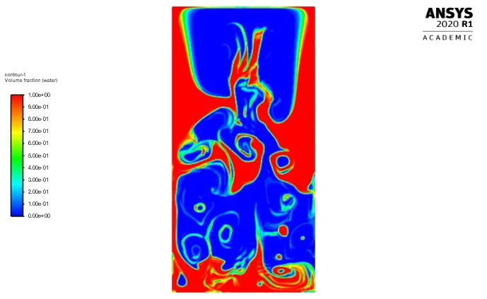
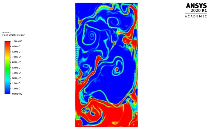
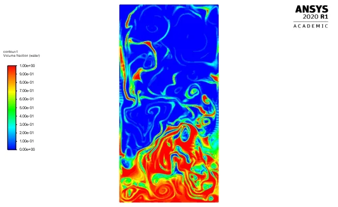
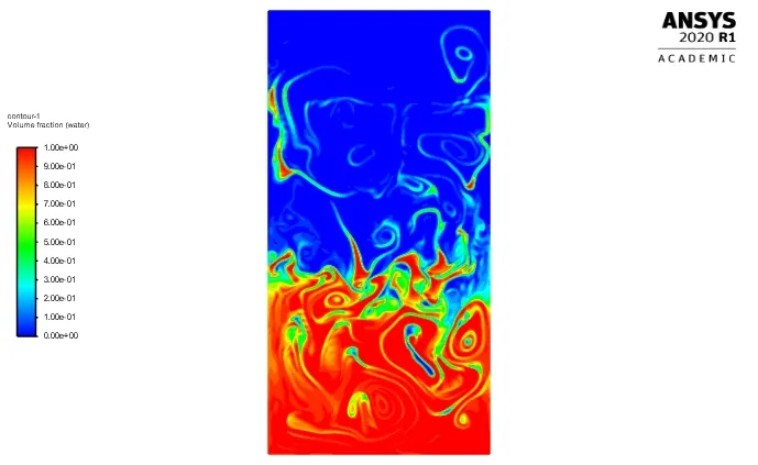
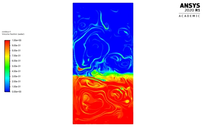
2. Contour plot of water-air volume fraction at different time ( 0.025s , 0.075s , 0.125s , 0.2s ,0.375s , 0.7s , 1.25s , 3s , 5s , 5.625s , 6.875s )

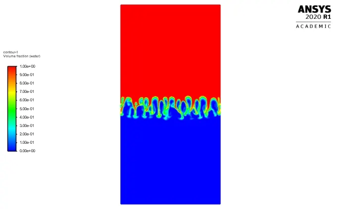
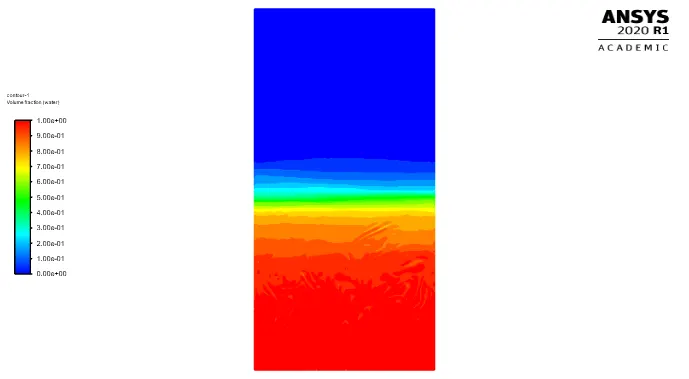
google drive link : https://drive.google.com/file/d/1N5Q6rjzKc9Czi9rmatV_7WKI95B6-7TL/view?usp=drivesdk

• For above case Atwood number is near about 0.99 because of high density differnece (999-1 =998 ) instantanous hydrostatic force devloped at fluids interface .
• for t= 0.025s intial small enough perturbation crated becauses of larges forces due to density differences results in spikes of high density fluid accerates downward which is in linear region
• we observed the transition of single globues of fluid deformed into lots of another globules which is vanished at time near 0.2s after that fluid starts to rolls up with displacing higher fluid completely downward side
• at time step near about t=2s fluid enters in non -linear region with increse in the amplitude of perturbation
• later time we observed small globules of low density fluid rise apward and same time globues of high density moves in downward and tried to settle down
• with the time evolution interface gets smeared due to numerical diffusion within the interfaces.

• CASE -2

• Mesh size 0.1mm for User_Defined material-water phase
  
  • No. of Nodes : 80601
  • No. of elements : 80000
  • Size of Time step : 0.025 & No. of Time- step :350

1. Residual plot

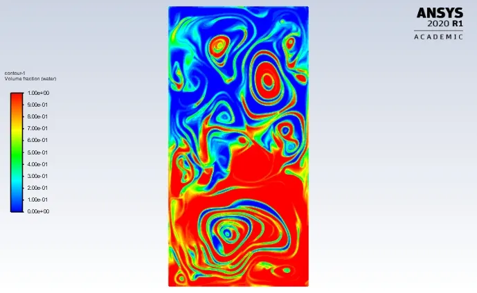
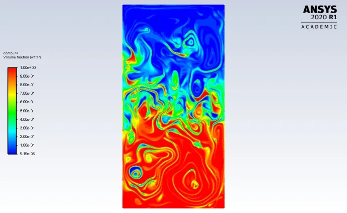
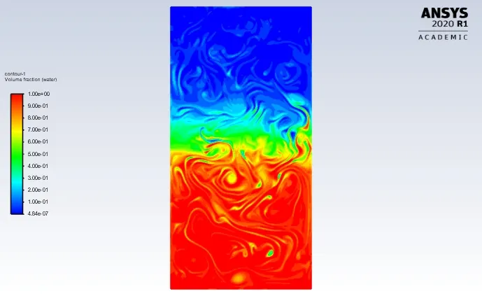
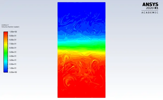
2. Contour plot of water-air volume fraction at different time ( 0.1s , 0.15s , 0.25s , 0.375s , 0.5s , 0.875s , 1.25s , 2s , 3.5s , 5s , 6.625, 8.75s )

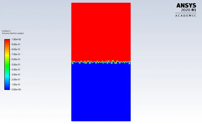
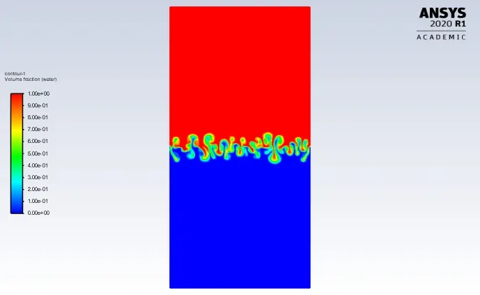
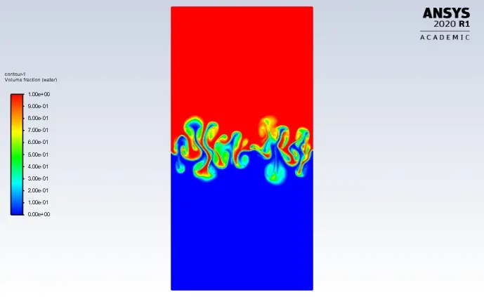
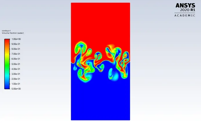
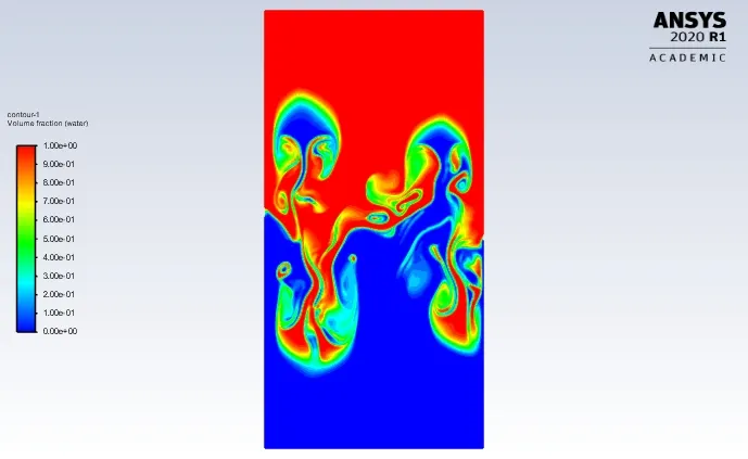
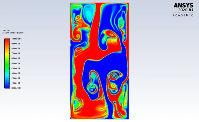
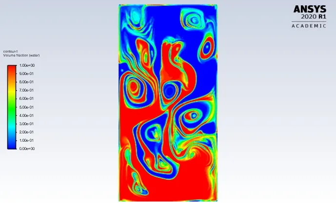
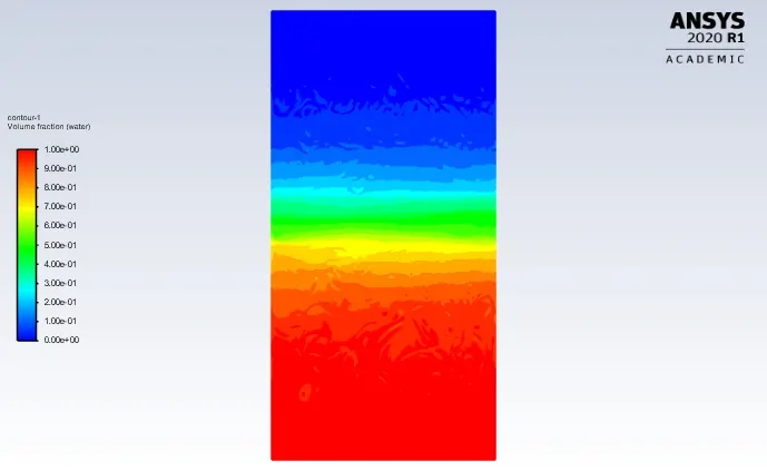
google drive link : https://drive.google.com/file/d/152hap1x4jFKCneQKDKWLVXR14QwmRPen/view?usp=drivesdk

• For above case Atwood number is near about 0.42 because of high density differnece (999-400 =599 ) instantanous hydrostatic force devloped at fluids interface .
• for t= 0.1 s intial small enough perturbation crated becauses of forces due to density differences (less compared to above case ) results in low spikes but more like bubble of high density fluid accerates downward which is in linear region
• we observed the transition of single globues of fluid deformed into lots of another globules which is vanished at time near 0.375s after that fluid starts to rolls up (t=0.875s) with displacing higher fluid completely downward side
• at time step near about t=3s fluid enters in non -linear region with increse in the amplitude of perturbation
• later time we observed small globules of low density fluid rise apward and same time globues of high density moves in downward and tried to settle down
• with the time evolution interface gets smeared due to numerical diffusion within the interfaces.

CONCLUSION

• The shape of globules actually varying with the time evolution which give better insight to understad phenomenon better as described above hence as its depend on time transient state is better then steady state condition
• with varying mesh size( Refined) final result of interface of complete settlling can be seen better as shown below and interface thickness is reduced

• increse in mesh size again leads to computation time cost as in here case for more fine mesh run for 350 time step whlie for corser mesh near about 120 .

• time for initial perturbation is different for different atwood no. ex, for atwood no = 0.99 due to high forces intial perturbation devloped more quickly at t=0.025s while for low atwood no. due to less forces ( low density differnce ) initial perturbation devloped at t= 0.1s
• At very due to large instantanous force its better to use momentum first order upwind scheme order to ensure stability again this scheme leads to accuracy loss compared to second order