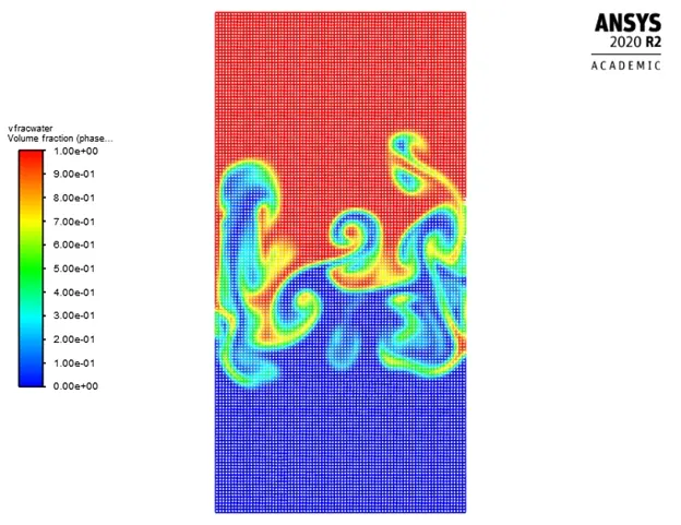
2D CFD analysis of Raylegih Taylor Instability.
Aim – Two dimensional CFD analysis of Rayleigh Taylor Instability.
Introduction –
The transition to turbulence begins usually with the instability of laminar state. This has been an area of interest from the last two centuries. Mathematicians and engineers have many a times offered remarkable insights from time to time.
Similar to oscillations of solids, a plethora of waves in fluids are available. Compressibility waves, gravity waves due to variation in buoyancy, inertial waves due to rotation etc. are a few of them.
Oscillations in fluids can be understood by a simple example. Consider a fluid at rest, whose density varies with depth i.e. the fluid is stably stratified. Now if a fluid parcel is displaced upwards, it is surrounded by lower density fluid and thus sinks. In the absence of retarding forces due to viscosity, it would then overshoot its mean position and reach a neighbourhood of fluid parcels of higher density. There it will experience an upward thrust. This oscillation will die down after some time.
Such wave like motion in fluids is abundant in nature. Ripples generated in a pond is an example of it.
However, now consider a fluid to be unstably stratified. The oscillations will increase and the parcel of fluid under study would accelerate away from its initial position. There are several flow instabilities which occur in nature. Some of these are given below –
Kelvin Helmholtz Instability (Effect of shear) – This is very commonly observed in nature. Consider two uniform streams of different velocities flowing past each other. This results in a shear force at the interface which results in a specific form of oscillation. This type of instability can easily be observed in clouds.
Rayleigh- Benard Flow (Effect of buoyancy) – One of the most easily realisable experiments on hydrodynamic instabilities is that of thermal convection. Consider a mass of fluid confined between two plates a distance H apart, held at different temperatures, with the bottom plate hotter than the top. We now have an unstable stratification, with lighter fluid below heavy, and the fluid therefore has a tendency to overturn. For small temperature differences, viscosity is able to curb this tendency, and heat is transferred by conduction. As the temperature difference ∆T across a layer increases, or the diffusivities of momentum or heat (the kinematic viscosity ν, and k, respectively) decrease, the Rayleigh number Ra = βg∆TH3/νk increases. Here, βis the coefficient of thermal expansion. At a particular Rayleigh number of 1708 for this geometry, convection sets in and one observes patterns in the form of rolls.
Taylor – Couette Flow (Effect of Rotation) - An adverse temperature gradient is a potentially unstable arrangement. Exploring the striking similarities between rotating and stratified flows, one can consider a fluid with unstable angular momentum “stratification”. Rayleigh noted this analogy and stated that a rotating fluid will be stable to axisymmetric disturbances if its angular momentum increases monotonically outwards. If the square of the angular momentum of a fluid parcel between two rotating cylinders decreases radially, then there would be a release of energy, resulting in instability.
Rayleigh – Plateau Instability (Effect of surface tension) – Surface tension always tries to bring a body to a state of minimum surface energy by minimizing its surface area. This phenomenon has been observed by everybody when the jet of water coming out of tap breaks into a sequence of drops.
Rayleigh – Taylor Instability (Effect of densities) - The Rayleigh–Taylor instability, or RT instability (after Lord Rayleigh and G. I. Taylor), is an instability of an interface between two fluids of different densities which occurs when the lighter fluid is pushing the heavier fluid. Examples include the behavior of water suspended above oil in the gravity of Earth, mushroom clouds like those from volcanic eruptions and atmospheric nuclear explosions, supernova explosions in which expanding core gas is accelerated into denser shell gas, instabilities in plasma fusion reactors etc.
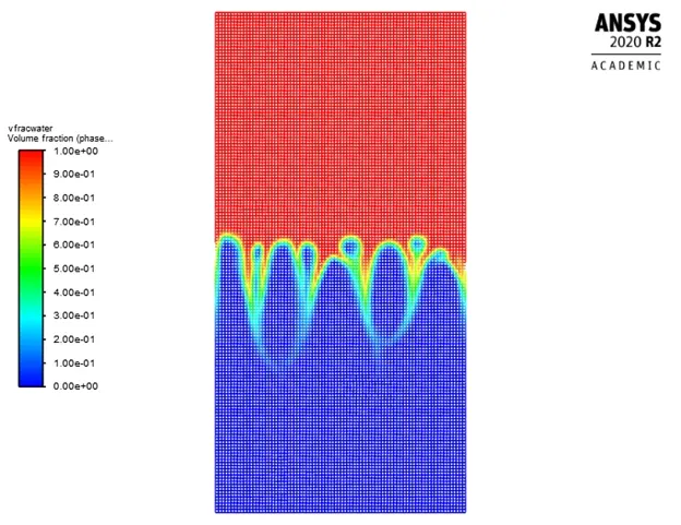
The evolution of the RTI follows four main stages. In the first stage, the perturbation amplitudes are small when compared to their wavelengths, the equations of motion can be linearized, resulting in exponential instability growth. In the early portion of this stage, a sinusoidal initial perturbation retains its sinusoidal shape. However, after the end of this first stage, when non-linear effects begin to appear, one observes the beginnings of the formation of the ubiquitous mushroom-shaped spikes (fluid structures of heavy fluid growing into light fluid) and bubbles (fluid structures of light fluid growing into heavy fluid). The growth of the mushroom structures continues in the second stage and can be modeled using buoyancy drag models, resulting in a growth rate that is approximately constant in time. At this point, nonlinear terms in the equations of motion can no longer be ignored. The spikes and bubbles then begin to interact with one another in the third stage. Bubble merging takes place, where the nonlinear interaction of mode coupling acts to combine smaller spikes and bubbles to produce larger ones. Also, bubble competition takes places, where spikes and bubbles of smaller wavelength that have become saturated are enveloped by larger ones that have not yet saturated. This eventually develops into a region of turbulent mixing, which is the fourth and final stage in the evolution. It is generally assumed that the mixing region that finally develops is self-similar and turbulent, provided that the Reynolds number is sufficiently large fusion reactors and inertial confinement fusion.
Apart from the instabilities mentioned above, there are many others.
Different models available for the CFD analysis of Rayleigh – Taylor instabilities are –
- Potential Flow Models
- Buoyancy drag models
- K –L two equation models
- K – L three equation models
- K-L four equation models
Modelling and Solving approach –
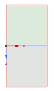
Solid Model – A 2D surface (2 surfaces) was sketched in Ansys Spaceclaim.
The Pull extraction feature of Spaceclaim was utilized to generate each of the surfaces and the topology was shared using the Share feature of Spaceclaim to get conformal mesh between the solid and fluid regions. The geometry was then exported to Ansys Mesher. The surface in Spaceclaim is shown below.
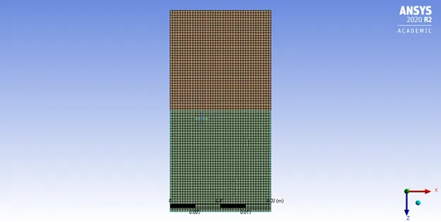
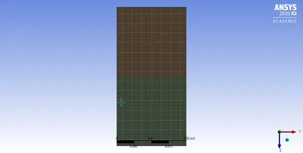
Meshing – Two different meshing strategies were utilized. The fluids were air and water in cases 1 and 2 while in the third case the fluids were water and a custom fluid. The mesh for case 2 and case 3 was the same.
The mesh statistics for all the cases are given in the below table.
|
|
Element size (mm) [element type] |
Number of elements |
|
Case 1 |
0.5 [Quadrilateral] |
3200 |
|
Case 2 |
0.25 [Quadrilateral] |
12800 |
|
Case 3 |
0.25 [Quadrilateral] |
12800 |
The images of the mesh domain for case 1 and 2 are given below –
Case 1
Case 2
Solver Settings – Ansys Fluent was used as the solver and transient simulations have been performed using a pressure based solver. The gravitational acceleration was taken as -9.81 m/s2.
Boundary conditions – No inlet and outlets were considered. All the boundaries of the domain were taken as wall.
Computational model – As the flow domain is quite small (each of the two surface is a square of 20 mm side) and the flow takes place purely due to the body force, laminar model has been chosen for the study.
Spatial Discretization Method – SIMPLE Pressure velocity coupling scheme was used to solve the Navier Stokes Equations. The methods used for spatial discretization of each of the terms is given in the below table –
|
Term/Equation |
Method |
|
Gradient |
Least Squares Cell based |
|
Pressure |
Second Order |
|
Momentum |
Second Order Upwind |
|
Time step size |
0.005 |
|
Number of time steps |
500 |
Results and Discussion –
The flow regime changes depend on the Atwood number. Atwood number is defined as -
`A= (ρ_1-ρ_2)/(ρ_1+ρ_2)`
Where
`ρ_1`is the density of heavier fluid
`ρ_2`is the density of lighter fluid
It is used in the study of hydrodynamic instabilities in density stratified flows.
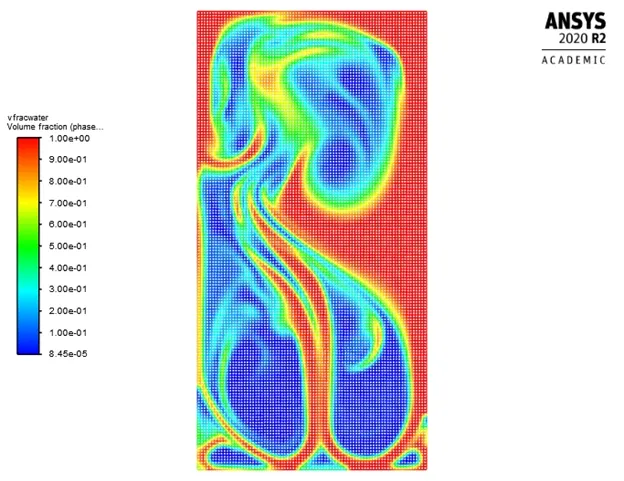
It is found that in lower Atwood number cases, the spike may disintegrate from the heavier fluid, while in the higher Atwood cases, the confined domain boundaries do not allow it to happen. In higher Atwood numbers, the secondary instabilities especially in the bubble region disappear. As the Atwood number increases, the spike stem and side-tails become narrower and sharper in shape.
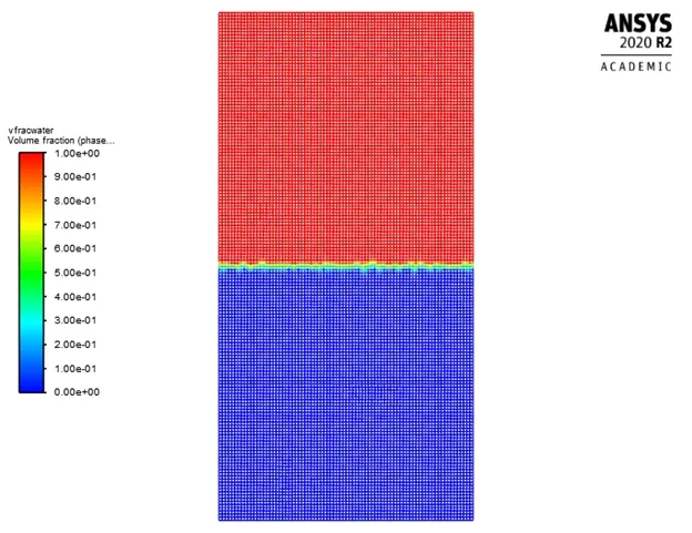
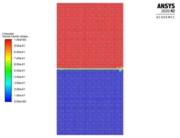
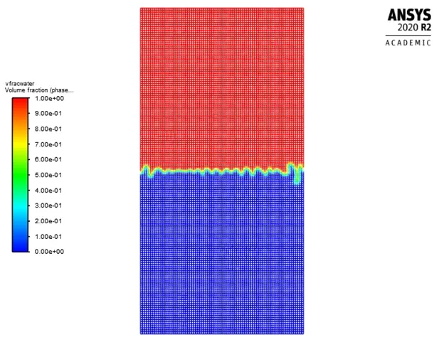
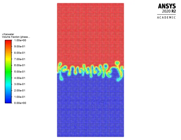
The snapshots of the major stages mentioned in the RT instability description above are shown below for case 2 and case 3. It is clear that the instability beginning at all the other stages are more delayed when Atwood number (A) is lesser.
Case 2 –
`A=(1000-1.225)/(1000+1.225)=0.9975`
The animation for this case can be viewed at -
https://www.youtube.com/watch?v=0DyESugSrdg
Onset of instability (Stage 1) at time step = 6
Mushroom shaped spikes (Stage 2) at time step = 13
Bubble competitions (Stage 3) at time step = 20 (coalescence at time step =25)
t = 20
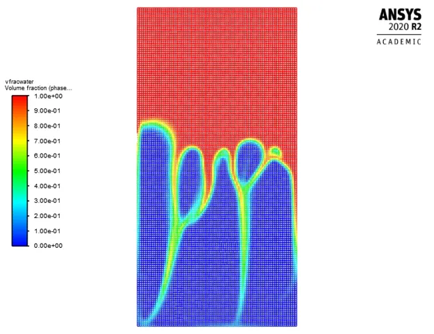
T = 25 (Bubble coalescence)
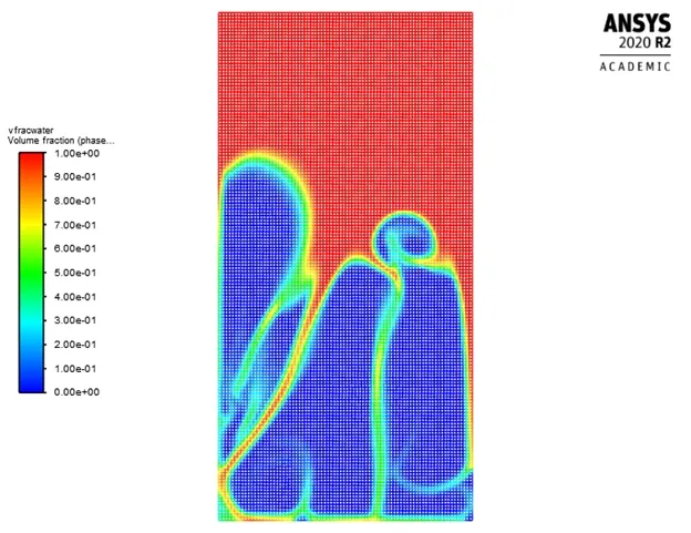
Onset of turbulent mixing (Stage 4) at time step = 50
Case 3 –
`A=(1000-400)/(1000+400)=0.4286`
The animation for this case can be viewed at -
https://www.youtube.com/watch?v=GH4-W4YqHJ0
Onset of instability (Stage 1) at time step = 23. Also shown below is a snapshot at time step = 28.
Disintegration of spikes (Stage 2) at time step = 37 indicating a less prominent mushroom effect
Onset of turbulent mixing at time step = 65