Rankine cycle simulator using MATLAB
AIM: To create a Rankine cycle simulator using MATLAB.
EQUATION: The formulae are as follows:
| Type | Enthalpy (kJ/kg) | Entropy (kJ/kgK) | Specific Volume (m^3/kg) |
| Liquid | `h = h_f` | `S = S_f` | `v = v_f` |
| Wet | `h = h_f + x.h_[fg]` | `S = S_f + x.S_[fg]` | `v = x.v_g` |
| Dry | `h = h_g` | `S = S_g` | `v = v_g` |
| Superheated | `h = h_g + Cp_s (T - T_[sat])` | `S = S_g + Cp_v .ln(frac[T][T_[sat]])` | `v = v_g . (frac[T][T_[sat]])` |
`Q_(out) = h_2 - h_3`
`W_T = h_1 - h_2`
`W_P = h_4 - h_3`
`Q_(i n) = h_1 - h_4`
`W_(n et) = W_T - W_P`
`eta_t = frac[W_(n et)][Q_(i n)]`
where;
`T` = Temeprature (K)
`T_[sat]` = Saturated Temeprature (K)
`W_T` = Work done on Turbine (kJ/kg)
`W_P` = Work done by Pump (kJ/kg)
`W_(n et)` = Net Work (kJ/kg)
`Q_(i n)` = Heat gained by Boiler (kJ/kg)
`Q_(out)` = Heat rejected by Condenser (kJ/kg)
`eta_t` = Thermal Efficiency
OBJECTIVE:
1. To calculate the state points of the Rankine Cycle (any type of your choice) based on user inputs:
Turbine Inlet temperature = 400° C
Turbine Inlet Pressure = 30 bar
Turbine Outlet Pressure = 0.05 bar = Condenser Inlet Pressure
2. To plot the corresponding T-S and h-S plots for the given set of inputs.
3. To calculate Net work output, Back work ratio and other parameters according to the given image below.
4. The main program should take the XSteam.m file as an input and generate the state points.
Sample Output:
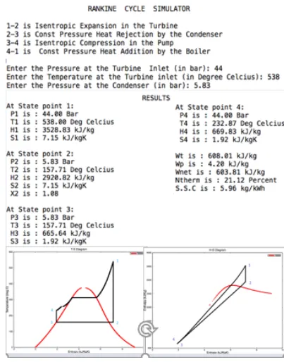
THEORY:
|
The Rankine cycle is an idealized thermodynamic cycle of a constant pressure heat engine that converts part of heat into mechanical work. In this cycle, the heat is supplied externally to a closed loop, which usually uses water (in a liquid and vapor phase) as the working fluid. In contrast to the Brayton cycle, the working fluid in the Rankine cycle undergo the phase change from a liquid to vapor phase and vice versa. Water is usually used as the working fluid due to its favorable properties, such as its non-toxic and unreactive chemistry, abundance, and low cost, as well as its thermodynamic properties. In case of the Rankine cycle, the Ideal Gas Law almost cannot be used (steam do not follow Pv=nRT), therefore all important parameters of water and steam are tabulated in so called "Steam Tables". One of the major advantages of the Rankine cycle is that the compression process in the pump takes place on a liquid. By condensing the working steam to a liquid (inside a condenser) the pressure at the turbine outlet is lowered and the energy required by the feed pump consumes only 1% to 3% of the turbine output power and these factors contribute to a higher efficiency for the cycle. |
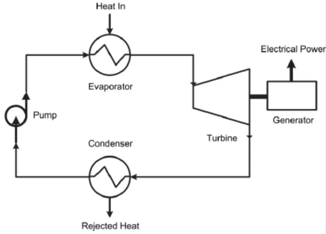 |
In an ideal Rankine cycle, the system executing the cycle undergoes a series of four processes:
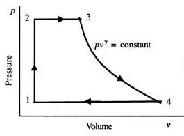
Process 1-2: Isentropic expansion (Turbine) – Steam from the boiler expands adiabatically in a steam turbine to produce work and then is discharged to the condenser (partially condensed). The steam does work on the surroundings (blades of the turbine) and loses an amount of enthalpy equal to the work that leaves the system. Again the entropy remains unchanged.
Process 2-3: Isobaric heat rejection (Condenser) – In this phase the cycle completes by a constant-pressure process in which heat is rejected from the partially condensed steam. There is heat transfer from the vapor to cooling water flowing in a cooling circuit. The vapor condenses and the temperature of the cooling water increases.
Process 3-4: Isentropic compression (Pump) – The liquid condensate is compressed adiabatically by centrifugal pumps (usually by condensate pumps and then by feedwater pumps). The liquid condensate is pumped from the condenser into the higher pressure boiler. In this process, the surroundings do work on the fluid, increasing its enthalpy and compressing it (increasing its pressure). On the other hand the entropy remains unchanged.
Process 4-1: Isobaric heat addition (Boiler) – In this phase, there is a constant-pressure heat transfer to the liquid condensate from an external source, since the chamber is open to flow in and out. The feedwater (secondary circuit) is heated from to the boiling point of that fluid and then evaporated in the boiler.
|
During the cycle, work is done on the fluid by the pump whereas work is done by the fluid in the turbine. The difference between the work done by the fluid and the work done on the fluid is the net work produced by the cycle and it corresponds to the area enclosed by the cycle curve (in PV diagram). The working fluid in a Rankine cycle follows a closed loop and is reused constantly. |
 |
SOLUTION:
Programming Language: MATLAB
Procedure/Steps:
1. Write the comments which you need at the beginning using fprintf command.
2. Use the input command to display the text in a prompt and assign the value when the user returns it.
3. To find the thermodynamic properties, XSteam command is used standard. It provides very accurate steam and water properties in ranges from 0-1000 bar and 0-2000°C.
(Temperature, Pressure, Enthalpy, Specific volume, Density, Specific entropy, Specific internal energy, Specific isobaric heat capacity, Specific isochoric heat capacity, Speed of sound, Viscosity, Vapour fraction)
4. Then add the thermodynamic relation to get the points in between the state variables.
5. Once all the state points are located, find the parameters like net work done, thermal efficiency, S.S.C., etc.
6. Display the calculated parameters as results using fprintf command.
7. Plot the saturation curves for both the liquid and steam phase using the for loop.
8. Finally, the state points are plotted using plot.
Code: The MATLAB program to visualize the Rankine cycle is shown below.
% Rankine Cycle Simulator.

fprintf('n           RANKINE CYCLE SIMULATOR n')
fprintf('1-2: Isentropic Expansion in the Turbine n')
fprintf('2-3: Constant Pressure Heat Rejection in the Condenser n')
fprintf('3-4: Isentropic Compression in the Pump n')
fprintf('4-1: Constant Pressure Heat Addition in the Boiler n')

% Inputs:

P1 = input('nEnter the Pressure at the Turbine Inlet (in bar): ')
T1 = input('Enter the Temperature at the Turbine Inlet (in Degree Celsius): ')
P2 = input('Enter the Pressure at the Condenser (in bar): ')


% Solution:

% High Pressure Line:
Tsat1 = XSteam('Tsat_p',P1);
Cpv1 = XSteam('CpV_p',P1);
Cpl1 = XSteam('CpL_p',P1);
Cpv4 = XSteam('CpV_p',P1);
Cpl4 = XSteam('CpL_p',P1);

% Point 1*:
hg1 = XSteam('hV_p',P1);
Sg1 = XSteam('SV_p',P1);

% Point 4*:
hf1 = XSteam('hL_p',P1);
Sf1 = XSteam('SL_p',P1);

% Low Pressure Line:
Tsat2 = XSteam('Tsat_p',P2);
Cpv2 = XSteam ('CpV_p',P2);
Cpl2 = XSteam ('CpL_p',P2);
Cpv3 = XSteam('CpV_p',P2);
Cpl3 = XSteam('CpL_p',P2);


% Point 2*:
hg2 = XSteam('hV_p',P2);
Sg2 = XSteam('SV_p',P2);

% Point 3:
hf2 = XSteam('hL_p',P2);
Sf2 = XSteam('SL_p',P2);

% State variables:
% Point 1:
h1 = XSteam('h_pT',P1,T1);
S1 = XSteam('S_pT',P1,T1);

% Point 2:
S2 = S1;
if (S2 <= Sg2)
    x2 = (S2-Sf2)/(Sg2-Sf2);
else
    x2 = 1;
end

if (x2 < 1)
    T2 = Tsat2;
    h2 = hf2 + x2*(hg2-hf2);
else
    % S2 = Sg2 + Cpv2*ln(T2+273/Tsat+273)
    T2 = ((Tsat2 + 273)*exp((S2-Sg2)/Cpv2)) - 273;
    h2 = hg2 + Cpv2*(T2 - Tsat2);
end

% Point 3: (No subcooling condition)
P3 = P2;
T3 = Tsat2;
h3 = hf2;
S3 = Sf2;
V3 = XSteam('vL_p',P3);

% Point 4:
P4 = P1;
S4 = S3;
Wp = (P4-P3)*V3*100;
% Wp = h4-h3;
h4 = h3+Wp;
% S4 = Sf1 + Cpl4*ln(T4/Tsat1)
T4 = (Tsat1*exp((S4-Sf1)/Cpl4));

Wt = h1-h2;
Wnet = Wt-Wp;
Qin = h1-h4;
Qout = h2-h3;
Ntherm = Wnet/Qin;
S.S.C = 3600/Wt;

% Saturation curve
T = linspace(1,373,50);
for i = 1:length(T)
    hl(i) = XSteam('hL_T',T(i));
    hv(i) = XSteam('hV_T',T(i));
    Sl(i) = XSteam('SL_T',T(i));
    Sv(i) = XSteam('SV_T',T(i));
end


% Output:

fprintf('     RESULTS n')
fprintf('nAt state point 1: n')
fprintf('P1 = %f bar n' ,P1)
fprintf('T1 = %f Degree Celsius n' ,T1)
fprintf('h1 = %f kJ/kg n' ,h1)
fprintf('S1 = %f kJ/kgK n' ,S1)

fprintf('nAt state point 2: n')
fprintf('P1 = %f bar n' ,P2)
fprintf('T2 = %f Degree Celsius n' ,T2)
fprintf('h2 = %f kJ/kg n' ,h2)
fprintf('S2 = %f kJ/kgK n' ,S2)

fprintf('nAt state point 3: n')
fprintf('P3 = %f bar n' ,P3)
fprintf('T3 = %f Degree Celsius n' ,T3)
fprintf('h3 = %f kJ/kg n' ,h3)
fprintf('S3 = %f kJ/kgK n' ,S3)

fprintf('nAt state point 4: n')
fprintf('P4 = %f bar n' ,P4)
fprintf('T4 = %f Degree Celsius n' ,T4)
fprintf('h4 = %f kJ/kg n' ,h4)
fprintf('S4 = %f kJ/kgK n' ,S4)

fprintf('nOther parameters: n')
fprintf('Wt = %f kJ/kg n', Wt)
fprintf('Wp = %f kJ/kg n', Wp)
fprintf('Wnet = %f kJ/kg n', Wnet)
fprintf('Ntherm = %f percent n', Wp)
fprintf('S.S.C = %f kg/kWhr n', S.S.C)


% Plot:

figure(1)
hold on
plot(Sl,T,'linewidth',2,'linestyle','--','color','b')
plot(Sv,T,'linewidth',2,'linestyle','--','color','k')
plot([S1 S2],[T1 T2],'linewidth',2,'color','r')
plot([Sg2 S3],[Tsat2 T3],'linewidth',2,'color','g')
plot([S3 S4],[T3 T4],'linewidth',2,'color','c')
plot([Sf1 Sg1],[Tsat1 Tsat1],'linewidth',2,'color','m')
plot([S2 Sg2],[T2 Tsat2],[Sg2 S3],[Tsat2 T3],'linewidth',2,'color','g')
plot([S4 Sf1],[T4 Tsat1],'linewidth',2,'color','m');
plot([Sg1 S1],[Tsat1 T1],'linewidth',2,'color','m');
text(S1,T1,' 1'); text(S2,T2,' 2'); text(Sg2,Tsat2,'  2*')
text(S3,T3,'3','HorizontalAlignment','right','VerticalAlignment','bottom')
text(S4,T4,'4','HorizontalAlignment','right','VerticalAlignment','bottom')
text(Sf1,Tsat1,' 4*','HorizontalAlignment','right','VerticalAlignment','bottom')
text(Sg1,Tsat1,' 1*')
xlabel('Entropy (kJ/kgK)')
ylabel('Temperature (Deg Celsuis)')
title('T-S diagram')
legend('Liquid curve','Vapour curve','Turbine','Condenser','Pump','Boiler')
grid on
hold off

figure(2)
hold on
plot(Sl,hl,'linewidth',2,'linestyle','--','color','b')
plot(Sv,hv,'linewidth',2,'linestyle','--','color','k')
plot([S1 S2],[h1 h2],'linewidth',2,'color','r')
plot([S2 S3],[h2 h3],'linewidth',2,'color','g')
plot([S3 S4],[h3 h4],'linewidth',2,'color','c')
plot([S4 S1],[h4 h1],'linewidth',2,'color','m')
text(S1,h1,' 1'); text(S2,h2,' 2')
text(S3,h3,'3','HorizontalAlignment','right','VerticalAlignment','top')
text(S4,h4,'4','HorizontalAlignment','right','VerticalAlignment','bottom')
xlabel('Entropy (kJ/kgK)')
ylabel('Enthalpy (kJ/kg)')
title('h-S diagram')
legend('Liquid curve','Vapour curve','Turbine','Condenser','Pump','Boiler')
grid on
hold off
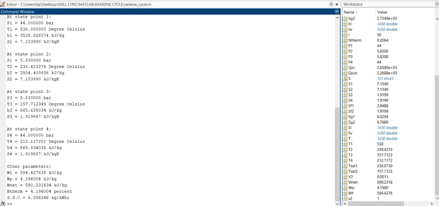
Output: The efficiencies are calculated and the problem is solved as shown below.
Command Window:
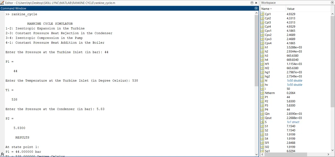
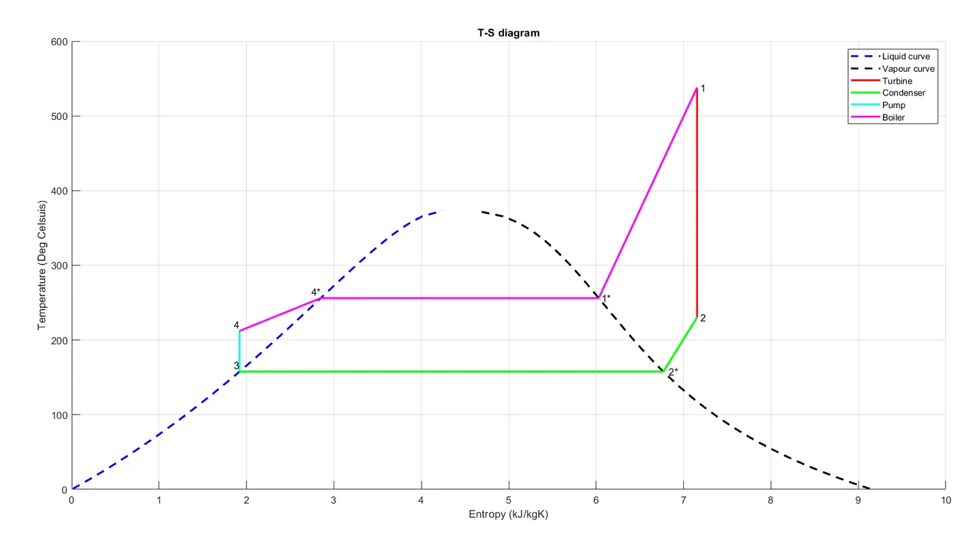
Plot: All the state points are plotted and connected according to their respective process nature as shown below.
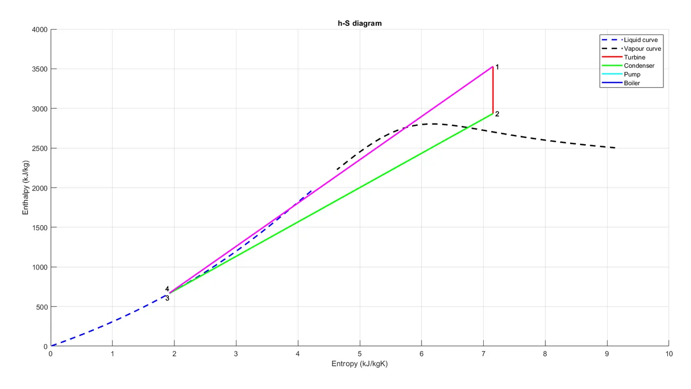
CONCLUSION: From the above results, we can see that the given problem statement is executed by calculating the thermodynamic properties and plotting the curves of all the species.
REFERENCES: XSteam.m file