Rankine cycle Simulator using MATLAB
AIM
To create a Rankine Cycle Simulator using MATLAB.
OBJECTIVES
- Calculate the state points of the Rankine Cycle.
- Plot the corresponding T-s and h-s plots of the Rankine Cycle.
- Get the steam table data for water from standard Xsteam library.
- Use steam table data to calculate the points in between the state variables.
- Calculate the work and effciency of the Rankine Cycle.
BASIC STUDY
The Rankine cycle comprises the following processes.
- Process 1-2: Reversible adiabatic expansion process in the steam turbine
- Process 2-3: Constant pressure heat transfer process in the condenser
- Process 3-4: Reversible adiabatic compression process in the pump.
- Process 4-1: Constant pressure heat transfer process in the boiler
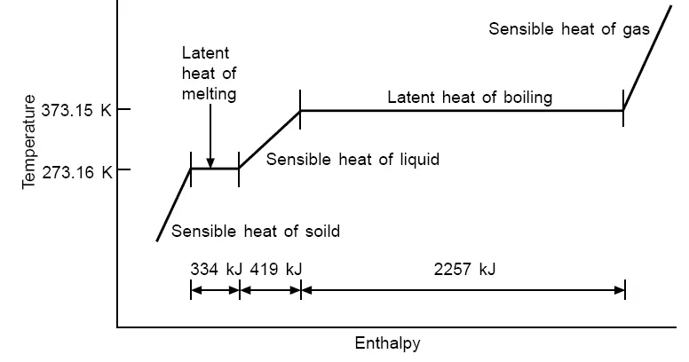
- Sensible Heat/Enthalpy of Water
- Latent Heat in Steam
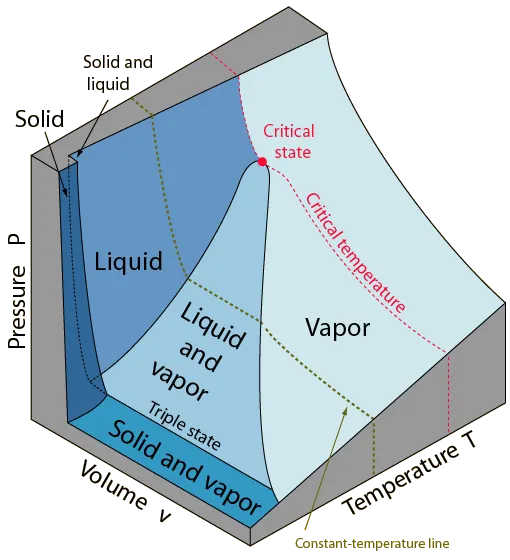
Critical state where the saturated-liquid and saturated-vapor lines meet. The state variables of this unique point are denoted by Pc, vc and Tc.
The remarkable "triple state" of matter where solid, liquid and vapor are in equilibrium may be characterized by a temperature called the triple point. The triple state is represented by a line parallel to the Pv plane with a characteristic pressure for the substance.
EQUATIONS
Calculating Work and Efficiency
Work transferred from the working fluid (kJ/kg)
`W_"turbine" = h1 - h2`
Heat rejected from the working fluid (kJ/kg)
`Q_"condenser" = h2 - h3`
Work transferred into the working fluid (kJ/kg)
`W_"pump" = h4 - h3`
Heat transferred to the working fluid (kJ/kg)
`Q_"boiler" = h1 - h4`
Back Work Ratio
`BWR = W_"turbine" / W_"pump"`
Specific Steam Consumption [kg/kWh]
`SSE = 3600/(W_"turbine" - W_"pump")`
Net work on the working fluid (kJ/kg)
`W_"net" = W_"turbine" - W_"pump"`
Rankine Cycle Efficiency
`eta_"rankine" = W_"net"/Q_"boiler"`
INPUT PARAMETERS
Turbine Inlet temperature = 400° C
Turbine Inlet Pressure = 30 bars
Turbine Outlet Pressure = 0.05 bars = Condenser Inlet Pressure
MATLAB PROGRAM
%% program to simulate Ideal Rankine cycle

% The Rankine cycle comprises the following processes.
% Process 1-2: Reversible adiabatic expansion process in the steam turbine
% Process 2-3: Constant pressure heat transfer process in the condenser
% Process 3-4: Reversible adiabatic compression process in the pump.
% Process 4-1: Constant pressure heat transfer process in the boiler

close all
clear all
clc

%% Inputs
t1 = 400;                                           % Turbine Inlet Temperature in [degree C]
p1 = 30;                                            % Turbine Inlet Pressure in [bar]
p2 = 0.05;                                          % Conderser Inlet Pressure in [bar]

%% State variable at state point 1
h1 = XSteam('h_pT',p1,t1);                          % Turbine Inlet Enthalpy in [kJ/kg]
s1 = XSteam('s_pT',p1,t1);                          % Turbine Inlet Specific entropy  in [kJ/kg K]
v1 = XSteam('v_pT',p1,t1);                          % Turbine Inlet Specific volume in [m3/kg]

%% State variable at state point 2
s2 = s1;                                            % Conderser Inlet Specific entropy  in [kJ/kg K]
h2 = XSteam('h_px',p2,XSteam('x_ps',p2,s2));        % Conderser Inlet Enthalpy in [kJ/kg]
t2 = XSteam('T_ps',p2,s2);                          % Conderser Inlet Temperature in [degree C]
v2 = XSteam('v_ps',p2,s2);                          % Conderser Inlet Specific volume in [m3/kg]

%% State variable at state point 3
p3 = p2;                                            % Pump Inlet Pressure in [bar]
t3 = XSteam('Tsat_p',p3);                           % Pump Inlet Temperature in [degree C]
h3 = XSteam('hL_p',p3);                             % Pump Inlet Enthalpy in [kJ/kg]
s3 = XSteam('sL_p',p3);                             % Pump Inlet Specific entropy  in [kJ/kg K]
v3 = XSteam('vL_p',p3);                             % Pump Inlet Inlet Specific volume in [m3/kg]

%% State variable at state point 4
s4 = s3;                                            % Boiler Inlet Specific entropy  in [kJ/kg K]
p4 = p1;                                            % Boiler Inlet Pressure in [bar]
h4 = XSteam('h_ps',p4,s4);                          % Boiler Inlet Enthalpy in [kJ/kg]
t4 = XSteam('T_ps',p4,s4);                          % Boiler Inlet Temperature in [degree C]
v4 = XSteam('v_ps',p4,s4);                          % Boiler Inlet Specific volume in [m3/kg]

%% Post Processing

%% Ploting path for Ideal Rankine cycle in T vs s Diagram
figure(1)
hold on
plot([s1 s2],[t1 t2],'color','g','linewidth',5);
plot([s2 s3],[t2 t3],'color','r','linewidth',5);
plot([s3 s4],[t3 t4],'color','m','linewidth',5);
Trange = linspace(t4,t1,100);
for i = 1:length(Trange)
    s_range(i) = XSteam('s_pT',p1,Trange(i));
    h_range23(i) = XSteam('h_ps',p1,s_range(i));
    h_range41(i) = XSteam('h_ps',p2,s_range(i));
end
plot(s_range,Trange,'color','b','linewidth',5);
legend('ReversibleAdiabaticExpansion', 'ConstantPressureHeatRejection', 'ReversibleIsentropicCompression', 'ConstantPressureHeatAddtion');

%% Ploting path for Ideal Rankine cycle in h vs s Diagram
figure(2)
hold on
plot([s1 s2],[h1 h2],'color','g','linewidth',5);
plot(s_range,h_range23,'color','r','linewidth',5);
plot([s3 s4],[h3 h4],'color','m','linewidth',5);
plot(s_range,h_range41,'color','b','linewidth',5);
legend('ReversibleAdiabaticExpansion', 'ConstantPressureHeatRejection', 'ReversibleIsentropicCompression', 'ConstantPressureHeatAddtion');

%% Ploting path for Ideal Rankine cycle in p vs v Diagram
figure(3)
hold on
p_range12 = linspace( p2,p1,100);
for i = 1:length(p_range12)
    v_range12(i) = XSteam('v_ps',p_range12(i),s1);
    v_range34(i) = XSteam('v_ps',p_range12(i),s3);
end
plot(v_range12,p_range12,'color','g','linewidth',5);
plot([v2 v3],[p2 p3],'color','r','linewidth',5);
plot(v_range34,p_range12,'color','m','linewidth',5);
plot([v4 v1],[p4 p1],'color','b','linewidth',5);
legend('ReversibleAdiabaticExpansion', 'ConstantPressureHeatRejection', 'ReversibleIsentropicCompression', 'ConstantPressureHeatAddtion');

%% Ploting T vs s Diagram for Water
t_range = linspace(0,374.15,500);                   % Temperature from 0 to critical point of water in [degree C]
figure(1)
hold on
for i = 1:length(t_range)
    plot(XSteam('sL_t',t_range(i)),t_range(i),'.','color','y')
    plot(XSteam('sV_t',t_range(i)),t_range(i),'.','color','y')
end

%% Ploting h vs s Diagram for Water
figure(2)
hold on
for i = 1:length(t_range)
    plot(XSteam('sL_t',t_range(i)),XSteam('hL_t',t_range(i)),'.','color','y')
    plot(XSteam('sV_t',t_range(i)),XSteam('hV_t',t_range(i)),'.','color','y')
end

%% Ploting p vs v Diagram for Water
figure(3)
hold on
grid on
for i = 1:length(t_range)
    plot(XSteam('vL_t',t_range(i)),XSteam('p_hs',XSteam('hL_t',t_range(i)),XSteam('sL_t',t_range(i))),'.','color','y')
    plot(XSteam('vV_t',t_range(i)),XSteam('p_hs',XSteam('hV_t',t_range(i)),XSteam('sV_t',t_range(i))),'.','color','y')
end

%% Ploting Diagram state points for Ideal Rankine cycle in T vs s
figure(1)
hold on
plot(s1,t1,'ko')
plot(s2,t2,'ko')
plot(s3,t3,'ko')
plot(s4,t4,'ko')
grid on
title('T-s Diagram of RANKINE CYCLE')
xlabel('Temperature in [degree C]')
ylabel('Specific entropy  in [kJ/kg K]')

%% Ploting Diagram state points for Ideal Rankine cycle in h vs s
figure(2)
hold on
plot(s1,h1,'ko')
plot(s2,h2,'ko')
plot(s3,h3,'ko')
plot(s4,h4,'ko')
grid on
title('h-s Diagram of RANKINE CYCLE')
xlabel('Enthalpy in [kJ/kg]')
ylabel('Specific entropy  in [kJ/kg K]')

%% Ploting Diagram state points for Ideal Rankine cycle in p vs v
figure(3)
hold on
plot(v1,p1,'ko')
plot(v2,p2,'ko')
plot(v3,p3,'ko')
plot(v4,p4,'ko')
grid on
title('p-v Diagram of RANKINE CYCLE')
xlabel('Specific volume in [m3/kg]')
ylabel('Pressure in [bar]')

%% Calculating Work and Efficiency
Wturbine = h1 - h2;                              % work transferred from the working fluid (kJ/kg)
Qcondenser = h2 - h3;                            % heat rejected from the working fluid (kJ/kg)
Wpump = h4 - h3;                                 % work transferred into the working fluid (kJ/kg)
Qboiler = h1 - h4;                               % heat transferred to the working fluid (kJ/kg)
BWR = Wturbine / Wpump;                          % Back Work Ratio
SSE = 3600/(Wturbine - Wpump);                   % Specific Steam Consumption [kg/kWh]
Wnet = Wturbine - Wpump;                         % Net work on the working fluid (kJ/kg)
ETArankine = Wnet/Qboiler;                       % Rankine Cycle Efficiency

clc
%% Printing Results to USER
fprintf('**********Program to simulate Ideal Rankine cycle**********\n\n');

fprintf('Process 1-2: Reversible adiabatic expansion process in the steam turbine\n');
fprintf('Process 2-3: Constant pressure heat transfer process in the condenser\n');
fprintf('Process 3-4: Reversible adiabatic compression process in the pump\n');
fprintf('Process 4-1: Constant pressure heat transfer process in the boiler\n\n');

fprintf('----------State variable at state point 1----------\n');
fprintf('Turbine Inlet Temperature T1 = %.4f in [degree C]\n',t1);
fprintf('Turbine Inlet Pressure p1 = %.4f in [bar]\n',p1);
fprintf('Turbine Inlet Enthalpy h1 = %.4f in [kJ/kg]\n',h1);
fprintf('Turbine Inlet Specific entropy s1 = %.4f in [kJ/kg K]\n',s1);
fprintf('Turbine Inlet Specific volume v1 = %.4f in [m3/kg]\n\n',v1);

fprintf('----------State variable at state point 2----------\n');
fprintf('Conderser Inlet Temperature T1 = %.4f in [degree C]\n',t2);
fprintf('Conderser Inlet Pressure p1 = %.4f in [bar]\n',p2);
fprintf('Conderser Inlet Enthalpy h1 = %.4f in [kJ/kg]\n',h2);
fprintf('Conderser Inlet Specific entropy s1 = %.4f in [kJ/kg K]\n',s2);
fprintf('Conderser Inlet Specific volume v1 = %.4f in [m3/kg]\n \n',v2);

fprintf('----------State variable at state point 3----------\n');
fprintf('Pump Inlet Temperature T1 = %.4f in [degree C]\n',t3);
fprintf('Pump Inlet Pressure p1 = %.4f in [bar]\n',p3);
fprintf('Pump Inlet Enthalpy h1 = %.4f in [kJ/kg]\n',h3);
fprintf('Pump Inlet Specific entropy s1 = %.4f in [kJ/kg K]\n',s3);
fprintf('Pump Inlet Specific volume v1 = %.4f in [m3/kg]\n \n',v3);

fprintf('----------State variable at state point 4----------\n');
fprintf('Boiler Inlet Temperature T1 = %.4f in [degree C]\n',t4);
fprintf('Boiler Inlet Pressure p1 = %.4f in [bar]\n',p4);
fprintf('Boiler Inlet Enthalpy h1 = %.4f in [kJ/kg]\n',h4);
fprintf('Boiler Inlet Specific entropy s1 = %.4f in [kJ/kg K]\n',s4);
fprintf('Boiler Inlet Specific volume v1 = %.4f in [m3/kg]\n \n',v4);

fprintf('----------Work and Efficiency----------\n');
fprintf('Work transferred from the working fluid Wturbine = %.4f in [kJ/kg]\n',Wturbine);
fprintf('Heat rejected from the working fluid Qcondenser = %.4f in [kJ/kg]\n',Qcondenser);
fprintf('Work transferred into the working fluid Wpump = %.4f in [kJ/kg]\n',Wpump);
fprintf('Heat transferred to the working fluid Qboiler = %.4f in [kJ/kg]\n \n',Qboiler);

fprintf('Back Work Ratio BWR = %.4f \n',BWR);
fprintf('Specific Steam Consumption SSE = %.4f in [kg/kWh] \n',SSE);
fprintf('Net work on the working fluid Wnet = %.4f in [kJ/kg] \n',Wnet);
fprintf('Rankine Cycle Efficiency ETArankine = %.4f %% \n\n',ETArankine*100);

fprintf('\n******************************END******************************\n');
%% END
EXPLANATION
Step 1: Get input values for the Rankine Cycle.
Step 2: Get the steam table data for water from standard `"MATLAB Xsteam"` library.
Step 3: Use steam table data to calculate the points in between the state variables.
Step 4: Calculate the state points of the Rankine Cycle.
Step 5: Plot the corresponding T-s and h-s plots of the Rankine Cycle.
Step 6: Calculate the work and effciency of the Rankine Cycle.
RESULT
Output
**********Program to simulate Ideal Rankine cycle**********

Process 1-2: Reversible adiabatic expansion process in the steam turbine
Process 2-3: Constant pressure heat transfer process in the condenser
Process 3-4: Reversible adiabatic compression process in the pump
Process 4-1: Constant pressure heat transfer process in the boiler

----------State variable at state point 1----------
Turbine Inlet Temperature T1 = 400.0000 in [degree C]
Turbine Inlet Pressure p1 = 30.0000 in [bar]
Turbine Inlet Enthalpy h1 = 3231.5710 in [kJ/kg]
Turbine Inlet Specific entropy s1 = 6.9233 in [kJ/kg K]
Turbine Inlet Specific volume v1 = 0.0994 in [m3/kg]

----------State variable at state point 2----------
Conderser Inlet Temperature T1 = 32.8755 in [degree C]
Conderser Inlet Pressure p1 = 0.0500 in [bar]
Conderser Inlet Enthalpy h1 = 2110.7082 in [kJ/kg]
Conderser Inlet Specific entropy s1 = 6.9233 in [kJ/kg K]
Conderser Inlet Specific volume v1 = 22.9511 in [m3/kg]

----------State variable at state point 3----------
Pump Inlet Temperature T1 = 32.8755 in [degree C]
Pump Inlet Pressure p1 = 0.0500 in [bar]
Pump Inlet Enthalpy h1 = 137.7651 in [kJ/kg]
Pump Inlet Specific entropy s1 = 0.4763 in [kJ/kg K]
Pump Inlet Specific volume v1 = 0.0010 in [m3/kg]

----------State variable at state point 4----------
Boiler Inlet Temperature T1 = 32.9452 in [degree C]
Boiler Inlet Pressure p1 = 30.0000 in [bar]
Boiler Inlet Enthalpy h1 = 140.7622 in [kJ/kg]
Boiler Inlet Specific entropy s1 = 0.4763 in [kJ/kg K]
Boiler Inlet Specific volume v1 = 0.0010 in [m3/kg]

----------Work and Efficiency----------
Work transferred from the working fluid Wturbine = 1120.8628 in [kJ/kg]
Heat rejected from the working fluid Qcondenser = 1972.9431 in [kJ/kg]
Work transferred into the working fluid Wpump = 2.9971 in [kJ/kg]
Heat transferred to the working fluid Qboiler = 3090.8088 in [kJ/kg]

Back Work Ratio BWR = 373.9816
Specific Steam Consumption SSE = 3.2204 in [kg/kWh]
Net work on the working fluid Wnet = 1117.8657 in [kJ/kg]
Rankine Cycle Efficiency ETArankine = 36.1674 %


******************************END******************************
CONCLUSION
- The state points of the Rankine Cycle are calculated by using the steam table data for water from standard `"MATLAB Xsteam"` library.
- T-s , h-s and p-v plots of the Rankine Cycle are plotted and the work and effciency of the Rankine Cycle are calculated.
REFERENCES
- What is Steam?
- STEAM THERMODYNAMICS
- PvT Surface for a Substance which Expands Upon Freezing
- Adiabatic Process
- RANKINE POWER GENERATION CYCLE
- Rankine Power Cycles
- VAPOUR POWER CYCLES
- X Steam, Thermodynamic properties of water and steam.
- Thermodynamic Properties of Water (Steam Tables)
- Properties of Steam