Rankine Cycle Simulator
Rankine Cycle
Aim:- To show graphical representation of rankine cycle
Theory:-
he Rankine cycle or Rankine Vapor Cycle is the process widely used by power plants such as coal fired power plant or nuclear reactor. In this mechanism, a fuel is used to produce heat within a boiler, converting water into steam which then expands through a turbine producing useful work. This process was developed in 1859 by Scottish engineer William J.M. Rankine. This is a thermodynamic cycle which converts heat into mechanical energy—which usually gets transformed into electricity by electrical energy generation.
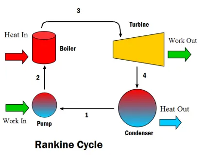
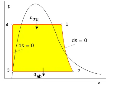
The steps in the Rankine Cycle as shown in Figure 1 and the corresponding steps in the volume diagram are outlined below:
- Pump: Compression of the fluid to high pressure using a pump (this takes work) ( Steps 3 to 4)
- Boiler: The compressed fluid is heated to the final temperature (which is at boiling point), therefore, a phase change occurs—from liquid to vapor. ( Steps 4 to 1)
- Turbine: Expansion of the vapor in the turbine. ( Steps 1 to 2)
- Condenser: Condensation of the vapor in the condenser (where the waste heat goes to the final heat sink (the atmosphere or a large body of water (ex. lake or river). Steps 2 to 3)
The efficiency of the Rankine cycle is limited by the high heat of vaporization by the fluid. The fluid must be cycled through and reused constantly, therefore, water is the most practical fluid for this cycle. This is not why many power plants are located near a body of water—that's for the waste heat.
Objective:- To get graphical representation of different phases of rankine cycle at different values of pressure,temperature,condemser pressure.
'XSteam.m' File link:- https://drive.google.com/file/d/1PcWvKQ9Ho4jTpwvvuZmluxw-PYX2_VWr/view?usp=sharing
Code:-
clear all
close all
clc

% Making Rankine Cycle Simulator
disp('Rankine Cycle')
disp('1-2: Isentropic Expansion')
disp('2-3: Isobaric Heat rejection by condenser')
disp('3-4: Isentropic Compression in Pump')
disp('4-1: Isobaric Heat Addition by the Boiler')
disp('')

t=linspace(0,373.15,200);

% Inputs factors
P1=input('Enter Pressure at turbine inlet:');
T1=input('Enter teperature at turbine inlet(Degree Celsius):');
P2=input('Enter pressure at condenser:');
disp('')

% State Point 1
h1=XSteam('h_pT',P1,T1);
s1=XSteam('s_pT',P1,T1);
hl1=XSteam('hL_p',P1);
hg1=XSteam('hV_p',P1);
sl1=XSteam('sL_p',P1);
sg1=XSteam('sV_p',P1);
Tsat1=XSteam ('Tsat_p',P1);

% State Point 2
s2=s1;
sl2=XSteam('sL_p',P2);
sg2=XSteam('sV_p',P2);

%Dryness Fraction
dry=(s2-sl2)/(sg2-sl2);


hl2=XSteam('hL_p',P2);
hg2=XSteam('hV_p',P2);
h2=hl2+dry*(hg2-hl2)
T2=XSteam('T_ph',P2,h2);
Tsat2=XSteam('Tsat_p',P2);

% State Point 3
h3=hl2
s3=sl2;
P3=P2;
T3=T2;

% State Point 4
s4=s3;
P4=P1;
h4=XSteam('h_ps',P4,s4)
T4=XSteam('T_ps',P4,s4);

% Plot of Temperature Vs Entropy
figure(1), clf
hold on

%Saturation Curve
for i=1:length(t)
    plot(XSteam('sL_T',t(i)),t(i),'r.')
    plot(XSteam('sV_T',t(i)),t(i),'r.')
end

% Cycle
plot([s1 s2],[T1 T2],'linewidth',2,'color','b')
text(s1,T1,'1','FontSize',15)

% Beyond saturation curve
if dry>1
    T3=Tsat2;
    plot([s2 sg2 s3 s4],[T2 Tsat2 T3 T4],'linewidth',2,'color','r')
    T2=Tsat2;
    text(s2,T2,'2','FontSize',15)
    text(s3,T3,'3','FontSize',15,'HorizontalAlignment','left','VerticalAlignment','top')

else
    plot([s2 s3 s4],[T2 T3 T4],'linewidth',2,'color','r')
    text(s2,T2,'2','FontSize',15)
    text(s3,T3,'3','FontSize',15,'HorizontalAlignment','left','VerticalAlignment','top')
end

n=linspace(T1,T2,500);
for i=1:length(n)
    plot(XSteam('s_pT',P1,n(i)),n(i),'.','linewidth',2,'color','g')
end

plot([sl1 sg1],[Tsat1 Tsat1],'linewidth',2,'color','b')
text(sl1,Tsat1,'4','FontSize',15,'VerticalAlignment','bottom')
xlabel('Entropy(kJ/kg-K)')
ylabel('Temperature(k)')
title('T-S Diagram')

% Enthsly Vs Entropy
figure(2), clf
hold on

%Saturation Curve
for i=1:length(t)
    plot(XSteam('sL_T',t(i)),XSteam('hL_T',t(i)),'r.')
    plot(XSteam('sV_T',t(i)),XSteam('hV_T',t(i)),'r.')
end

% Cycle
plot([s1 s2 s3 s4 s1],[h1 h2 h3 h4 h1],'linewidth',2,'color','b')
text(s1,h1,'1','FontSize',15)
text(s2,h2,'2','FontSize',15)
text(s3,h3,'3','FontSize',15)
text(s4,h4+90,'4','FontSize',15)

xlabel('Entropy(kJ/kg)')
ylabel('Enthalpy(kJ/kg)')
title('h-s Diagram')

% Calculation
work_turbine=h1-h2;
work_pump=h4-h3;
work_net=work_turbine-work_pump;
n_thermal=(1-((h2-h3)/(h1-h4)))*100;
bwr=work_pump/work_turbine;

ssc=3600/work_turbine;

disp('Result')

disp('At State Point 1:')                      # Phase 1 Point
fprintf('p1=%.2f abrn',P1)
fprintf(['t1=%.2f' char(176) 'Cn'],T1)
fprintf('h1=%.2f kJ/kgn',h1)
fprintf('s1=%.2f kJ/kgn',s1)
disp('')

disp('At State Point 2:')                    # Phase 2 Point
fprintf('p2=%.2f abrn',P2)
fprintf(['t2=%.2f' char(176) 'Cn'],T2)
fprintf('h2=%.2f kJ/kgn',h2)
fprintf('s2=%.2f kJ/kgn',s2)
disp('')

disp('At State Point 3:')                   # Phase 3 Point
fprintf('p3=%.2f abrn',P3)
fprintf(['t3=%.2f' char(176) 'Cn'],T3)
fprintf('h3=%.2f kJ/kgn',h3)
fprintf('s3=%.2f kJ/kgn',s3)
disp('')

disp('At State Point 4:')                 # Phase 4 Point
fprintf('p4=%.2f bar',P4)
fprintf(['t4=%.2f' char(176) 'Cn'],T4)
fprintf('h4=%.2f kJ/kg',h4)
fprintf('s4=%.2f kJ/kg',s4)
disp('')

fprintf('Work done by turbine=%.2f kJ/kg',work_turbine)
fprintf('Work done by pump=%.2f kJ/kg',work_pump)
fprintf('Net Work done=%.2f kJ/kg',work_net)
fprintf('Efficiency=%.2f %%n',n_thermal)
fprintf('Back work ratio=%f',bwr)
fprintf('Specific Steam Conductivity=%.2f kJ/kWh',ssc)
Explaination Of Code:-
P1,T1,P2 are taken as input values and t is assigned linspace command
XSteam file is imported and used for assigning different values
Different phase points are assigned with their values to plot on graph
formula for work of turbine,work of pump,thermal efficiency is given and calculated
Temperature Vs Entropy curve is plotted
Then Enthalpy Vs Entropy curve is plotted
Output:-
Output Values:-
Error Faced:-
Error cleared by using capital p instead of small p.
Conclusion:-
It can be concluded that rankine cycle depends on the fuel used as a source and also it changes value of thermal efficiency if source is changed.