RADIOSS Material Laws Challenge | HyperMesh

OBJECTIVE :

• To work on material card in Radioss and implement the different Material laws on the given component.
• To apply the seven different cases and compare them in a tabulated format.
• To compare total number of cycles, energy error, mass error and simulation time of all the cases.
• To notice the analysis animations of different cases and describe them in brief.
• To list down case by case result and conclusion for the cause of failure.

CASE SETUP AND EXECUTION :

The given model is as follows,

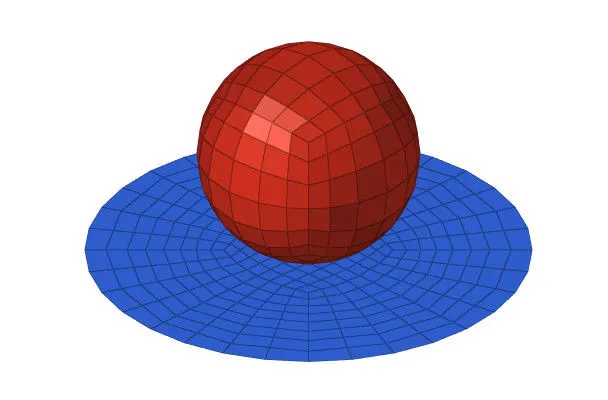
CASE 1 – Run the FAILURE_JOHNSON_0000 model as it is.

Steps to perform for this particular case;

Step I. In Radioss, Import FAILURE_JOHNSON_0000.rad starter file using Import Solver Deck menu.

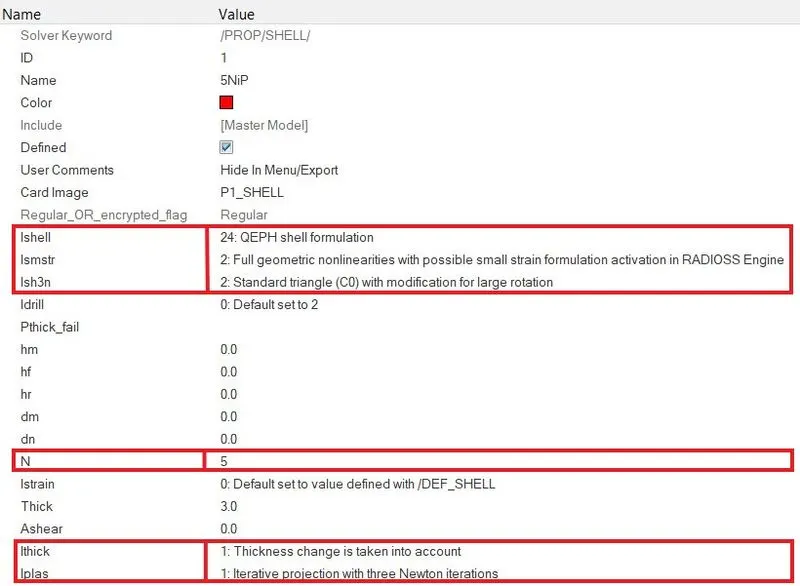
Step II. Change the properties of 5Nip to recommended properties which are given below.

Parameter	Comment
Ishell = 24	QEPH 4 nodes shells are best combination of cost and accuracy.
Ismstr = 2	Full geometric nonlinearities with possible small strain formulation.
Ish3n = 2	Standard 3 noded shell (C0) with modification for large rotation.
N = 5	Number of integration points set to 5 for accuracy bending.
Ithick = 1	Thickness change is taken into account for accuracy.
Iplas = 1	Iterative plasticity for good accuracy.

Step III. Navigate to Radioss panel in Analysis page.

Step IV. Save the model as Law2_epsmax_failure_0000.rad in a specific folder path, tick the include connectors option and under options folder write –nt 4 and click on Radioss to run the simulation.

Step V. Open .out Engine file from specified path and check final value of Energy error and mass error and check the values of Simulation time and Total number of cycles.

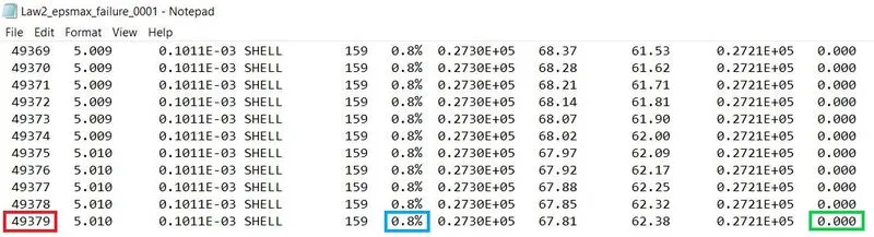
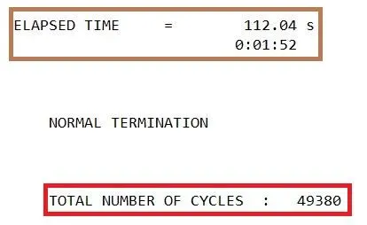
In the above images, red box indicates the Total number of cycles, blue box indicates Energy error, green box indicates Mass error and brown box indicates Simulation time.

Step VI. Open new model and switch to HyperView from Hypermesh.

Step VII. Load .h3d file from specified path, play the animation and plot contour of Von Mises stress using Simple averaging method.

Step VIII. Open HyperGraph 2D in a new window, load T01 file and plot the energies required.

Animation and Results –

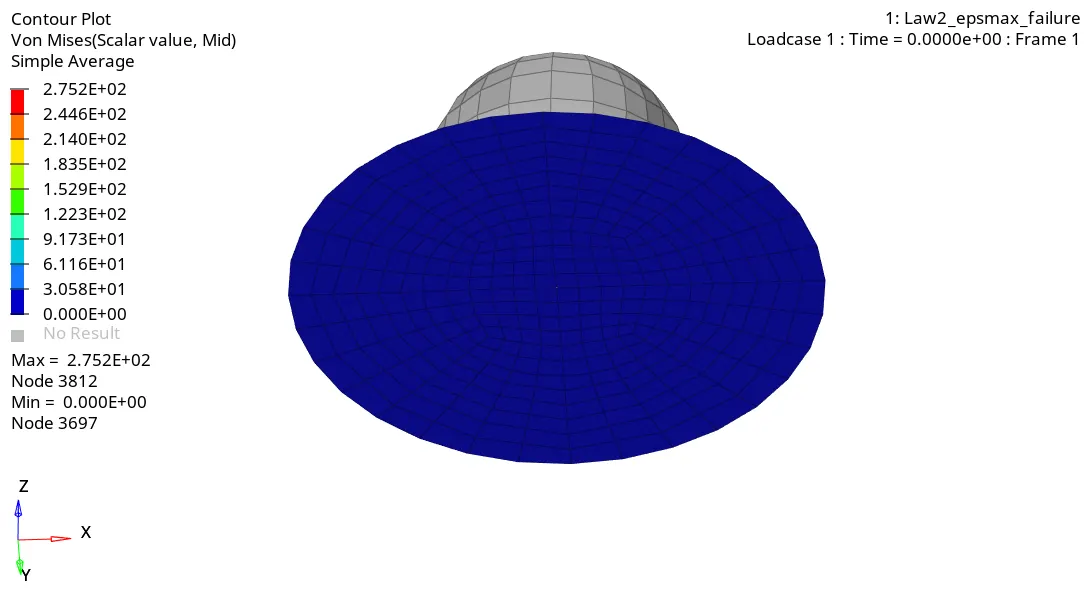
In this model, the Law2 material card is used which represents an isotropic elasto-plastic material using the Johnson-Cook material model. As the Law2 material card is used, the material will follow elastic-plastic behavior so after some initial stress, the SHELL4N component goes into plasticity and breaks. In LAW2, the maximum plastic strain Eps_p_max is used for element failure. This means the shell element is deleted once it reaches the maximum plastic strain defined in the model. Thus, initially the formation of crack is even and then we can see some elements getting deleted which results in uneven material removal. The other main reason for element deletion is due to the value of Ixfem which is zero, meaning it is deactivated.

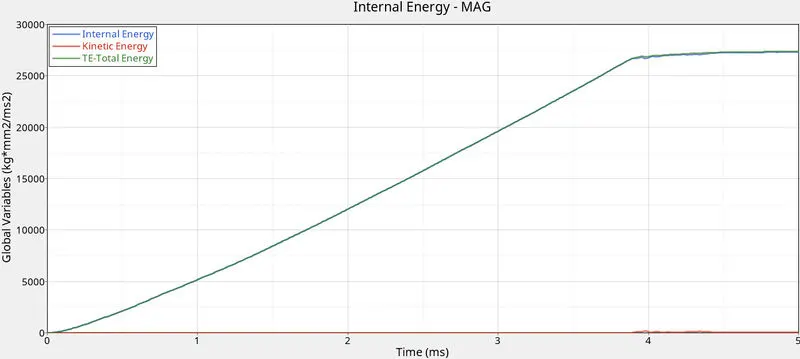
From the above energy plot, we can conclude that the internal energy and total energy of the model is almost the same as there is very less amount of kinetic energy in the model at the later stage.

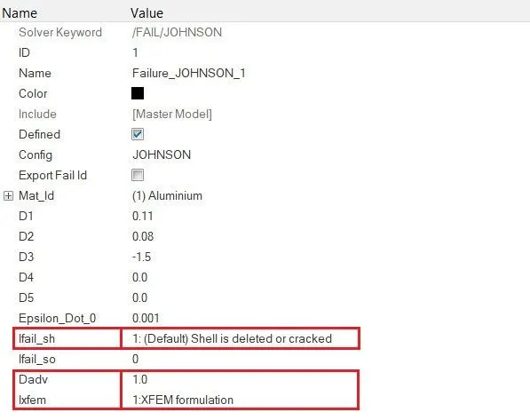
CASE 2 – In /FAIL/JOHNSON, change Ifail_sh=1, Dadv=1 and Ixfem=1.

Steps to perform for this particular case;

Step I. In Radioss, Import FAILURE_JOHNSON_0000.rad starter file using Import Solver Deck menu.

Step II. Open Failure_JOHNSON_1 under Failures card.

Step III. Do the changes as shown below.

Step IV. Navigate to Radioss panel in Analysis page.

Step V. Save the model as Law2_epsmax_crack_0000.rad in a specific folder path, tick the include connectors option and under options folder write –nt 4 and click on Radioss to run the simulation.

Step VI. Open .out Engine file from specified path and check final value of Energy error and mass error and check the values of Simulation time and Total number of cycles in the same way as mentioned in the previous case.

The values of Energy error, Mass Error, Simulation time and Total number of cycles are mentioned in tabulated format for all cases in Results.

Step VII. Open new model and switch to HyperView from Hypermesh. Load .h3d file from specified path, play the animation and plot contour of Von Mises stress using Simple averaging method.

Step VIII. Open HyperGraph 2D in a new window, load T01 file and plot the energies required.

Animation and Results –

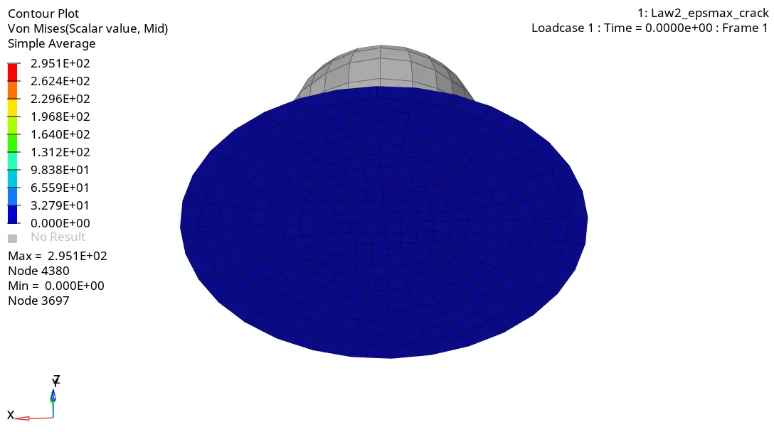
After making the changes to the model, we can observe that the elements are getting cracked at the initial stage. This cracking of elements is mainly developed due to Ixfem value which is set as 1. The value of Ifail_sh and Dadv is taken as default value when set to 1 or zero which impacts in shell failure and crack advancement when Ixfem is set to 1. Thus the elements are getting cracked.

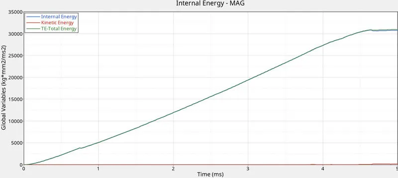
The internal energy is higher compared to previous case due to the cracking of elements.

CASE 3 – Delete the /FAIL/JOHNSON card and run the model.

Steps to perform for this particular case;

Step I. In Radioss, Import FAILURE_JOHNSON_0000.rad starter file using Import Solver Deck menu.

Step II. Open Failure_JOHNSON_1 under Failures card and delete it using delete button.

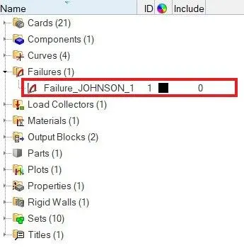
Step III. Navigate to Radioss panel in Analysis page.

Step IV. Save the model as Law2_epsmax_nofail_0000.rad in a specific folder path, tick the include connectors option and under options folder write –nt 4 and click on Radioss to run the simulation.

Step V. Open .out Engine file from specified path and check final value of Energy error and mass error and check the values of Simulation time and Total number of cycles in the same way as mentioned in the previous case.

Step VI. Open new model and switch to HyperView from Hypermesh. Load .h3d file from specified path, play the animation and plot contour of Von Mises stress using Simple averaging method.

Step VII. Open HyperGraph 2D in a new window, load T01 file and plot the energies required.

Animation and Results –

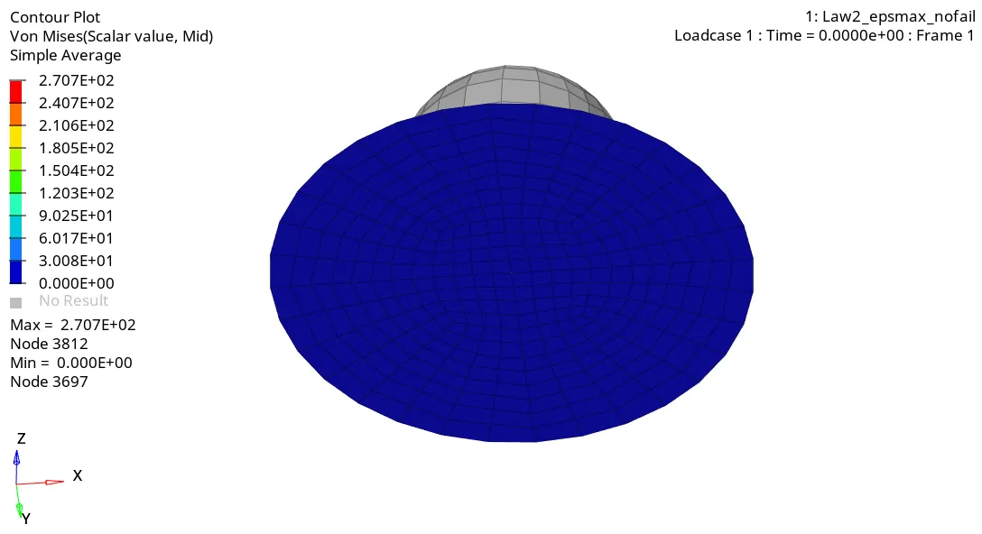
The simulation results for this model are same as Case 1 model. This is because of the LAW2(PLAS_JOHNS). This law contains a built-in failure criterion based on the maximum plastic strain which is almost the same for ductile materials. Thus even after deleting the /FAIL/JOHNSON card, we can see almost same results. The elements are deleted in very similar manner and the Von Mises Stress value is a bit high than the model with failure card.

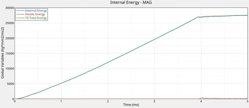
The energy plot above is same as we have got for the Case 1 model. Thus energy dissipation is also the same in both the cases.

CASE 4 – Delete the value of Eps_p_max and run the model.

Steps to perform for this particular case;

Step I. In Radioss, Import FAILURE_JOHNSON_0000.rad starter file using Import Solver Deck menu.

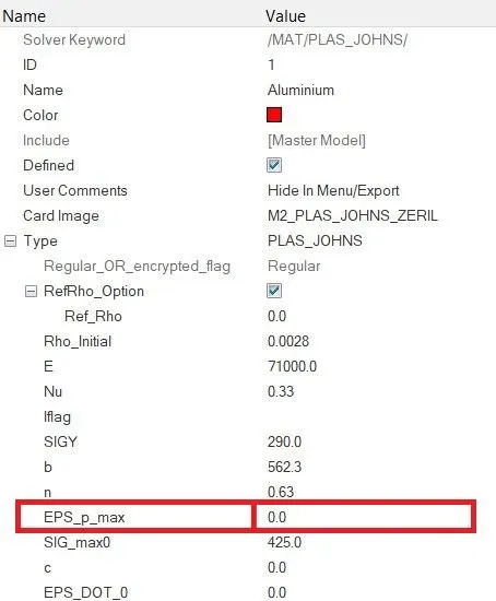
Step II. Open Aluminium material card under Materials and delete the value of Eps_p_max or enter the value as zero.

Step III. Navigate to Radioss panel in Analysis page.

Step IV. Save the model as Law2_ 0000.rad in a specific folder path, tick the include connectors option and under options folder write –nt 4 and click on Radioss to run the simulation.

Step V. Open .out Engine file from specified path and check final value of Energy error and mass error and check the values of Simulation time and Total number of cycles in the same way as mentioned in the previous case.

Step VI. Open new model and switch to HyperView from Hypermesh. Load .h3d file from specified path, play the animation and plot contour of Von Mises stress using Simple averaging method.

Step VII. Open HyperGraph 2D in a new window, load T01 file and plot the energies required.

Animation and Results –

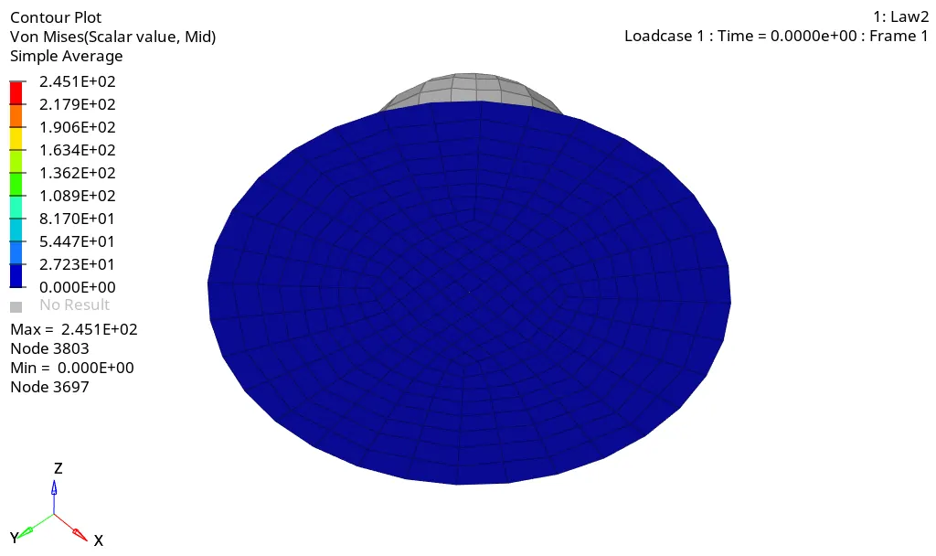
Based on the above animation, we can say that the PUNCH component doesn’t break into pieces as we have seen in the earlier cases. The failure happens only at the center and then it propagates evenly. This is due to the value of Eps_p_max which is defined as zero. So the software will take the default value 10³⁰ which means that the material is not going to fail under plastic strain. Since we have the Failure_JOHNSON card defined in the model, the material fails as shown in animation. We can also see some elements getting deleted as the Ixfem value is set to zero.

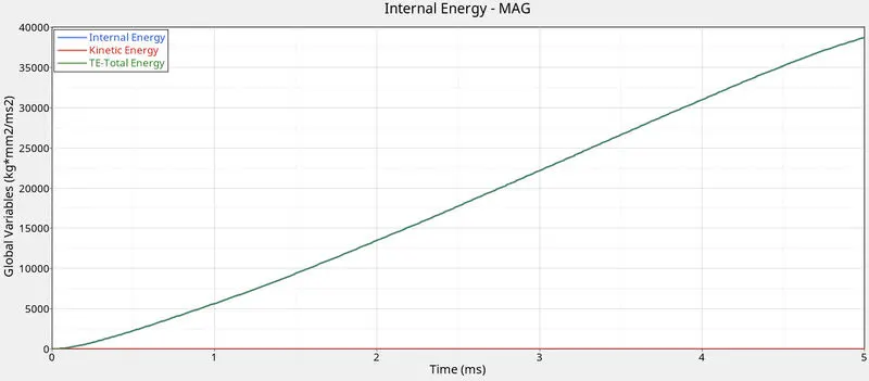
The internal and total energy of the model keeps on increasing linearly with time. Comparing above cases, the graph doesn’t become constant or the slope of the graph doesn’t bend to X-axis because the breaking of elements doesn’t happen.

CASE 5 – Convert the material model to Law1 Elastic with same parameter values.

Steps to perform for this particular case;

Step I. In Radioss, Import FAILURE_JOHNSON_0000.rad starter file using Import Solver Deck menu.

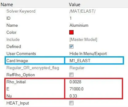
Step II. Open Aluminium material card under Materials and change the card image from M2_PLAS_JOHNS_ZERIL to M1_ELAST.

Step III. Enter the same values of Rho_initial, E and Nu which were in Law2 material card.

Step IV. Navigate to Radioss panel in Analysis page.

Step V. Save the model as Law1_ 0000.rad in a specific folder path, tick the include connectors option and under options folder write –nt 4 and click on Radioss to run the simulation.

Step VI. Open .out Engine file from specified path and check final value of Energy error and mass error and check the values of Simulation time and Total number of cycles in the same way as mentioned in the previous case.

Step VII. Open new model and switch to HyperView from Hypermesh. Load .h3d file from specified path, play the animation and plot contour of Von Mises stress using Simple averaging method.

Step VIII. Open HyperGraph 2D in a new window, load T01 file and plot the energies required.

Animation and Results –

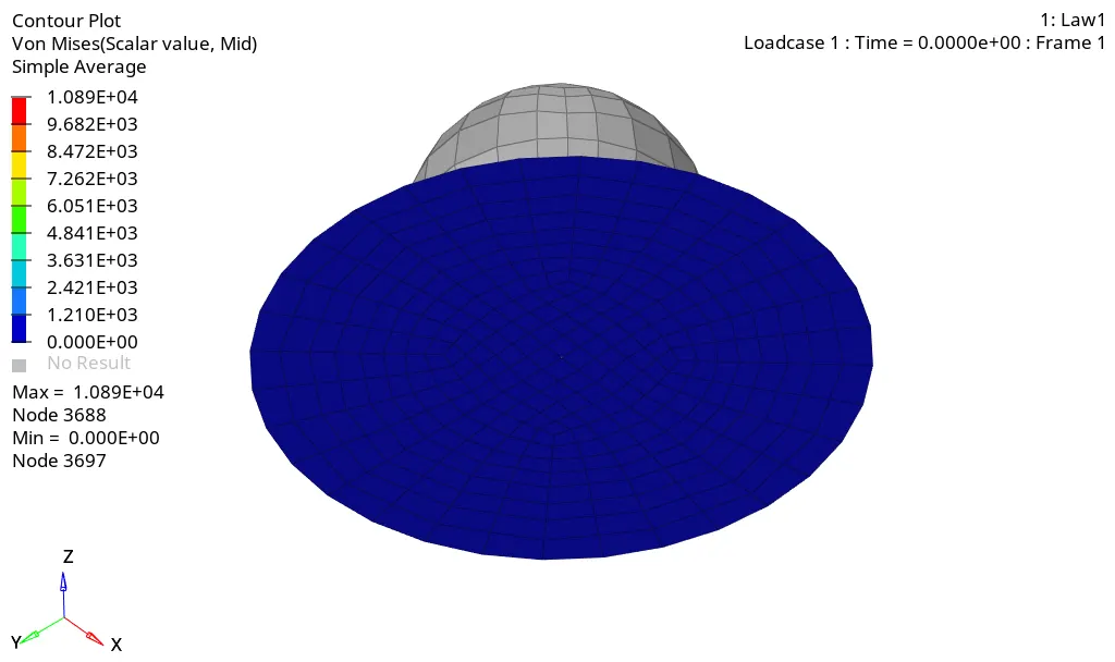
As the PUNCH component is defined elastic, the component characteristics will be in the elasticity zone and it won’t go in plastic deformation. Thus there is no failure in the simulation and the maximum stress is generated at the contact area between both the components. We can see some material penetrating through the PUNCH component as the contact between them is not defined properly.

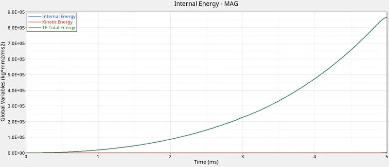
There is a very high amount of internal and total energy in the model as the material is elastic and high amount of energy is required to overcome the elasticity of the material.

CASE 6 – Open LAW27_0000.rad, change the shell properties to recommended shell properties and run.

Steps to perform for this particular case;

Step I. In Radioss, Import LAW27_0000.rad starter file using Import Solver Deck menu.

Step II. Change the properties of 5Nip to recommended properties which are used in Case 1.

Step III. Navigate to Radioss panel in Analysis page.

Step IV. Save the model as Law27_ 0000.rad in a specific folder path, tick the include connectors option and under options folder write –nt 4 and click on Radioss to run the simulation.

Step V. Open .out Engine file from specified path and check final value of Energy error and mass error and check the values of Simulation time and Total number of cycles in the same way as mentioned in the previous case.

Step VI. Open new model and switch to HyperView from Hypermesh. Load .h3d file from specified path, play the animation and plot contour of Von Mises stress using Simple averaging method.

Step VII. Open HyperGraph 2D in a new window, load T01 file and plot the energies required.

Animation and Results –

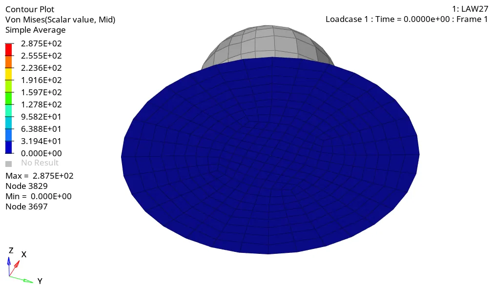
In this model, we used LAW27 which combines an isotropic elasto-plastic Johnson-Cook material model with an orthotropic brittle failure model. Thus we can see the brittle failure in the simulation. A group of elements is breaking or failing like failure in a brittle material. We can also see some elements getting deleted. This is because we have defined EPS_f1 and EPS_f2 value which monitors Maximum tensile strain for element deletion in principal strain direction.

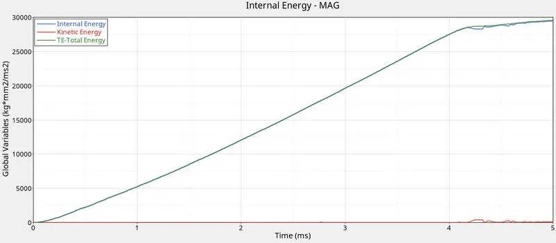
For energies plot, we can see some amount of kinetic energy being generated at the point of brittle failure. So the total energy plot deviates from internal energy plot. But the energy plot is almost similar to Law2 energy plot.

CASE 7 – Change the material card of FAILURE_JOHNSON_0000.rad to Law36 from Law2. Prepare and assign a curve to it and run the simulation.

Steps to perform for this particular case;

Step I. In Radioss, Import FAILURE_JOHNSON_0000.rad starter file using Import Solver Deck menu.

Step II. Open Aluminium material card under Materials and change the card image from M2_PLAS_JOHNS_ZERIL to M36_PLAS_TAB.

Step III. Under Curves card, create a new curve and name it as Plastic-True-Stress-Strain-Curve having the following coordinate values.

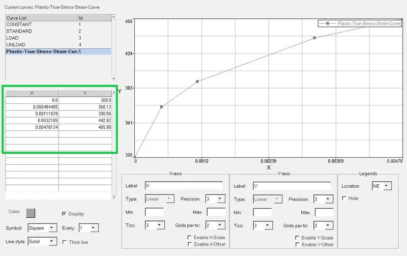
Step IV. Again navigate to Aluminium material card under Materials and enter the following values.

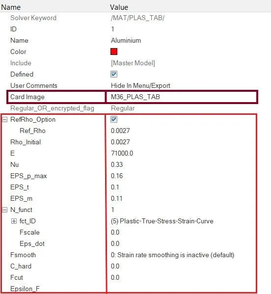
Step V. Navigate to Radioss panel in Analysis page.

Step VI. Save the model as Law36_ 0000.rad in a specific folder path, tick the include connectors option and under options folder write –nt 4 and click on Radioss to run the simulation.

Step VII. Open .out Engine file from specified path and check final value of Energy error and mass error and check the values of Simulation time and Total number of cycles in the same way as mentioned in the previous case.

Step VIII. Open new model and switch to HyperView from Hypermesh. Load .h3d file from specified path, play the animation and plot contour of Von Mises stress using Simple averaging method.

Step IX. Open HyperGraph 2D in a new window, load T01 file and plot the energies required.

Animation and Results –

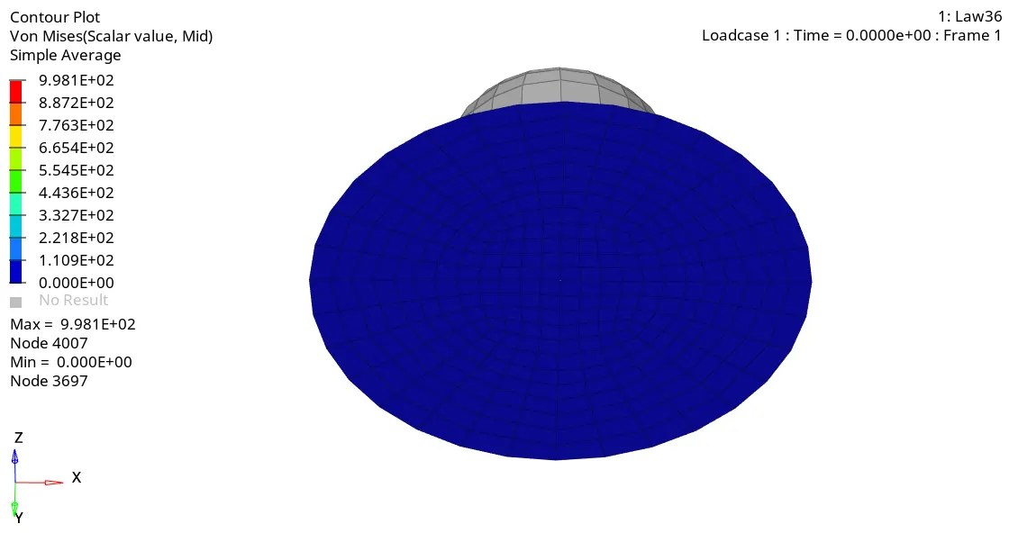
The Law36 models an isotropic elasto-plastic material using user-defined functions. Thus the failure in this model acts according to the curve which we defined. This type of failure represents the real life or true failure of the model as the failure parameters are testing and lab based. We can see that the material breaks at higher stress value which means that the material has lower value of plastic strain for higher value of stress which is the characteristic of true stress strain curve.

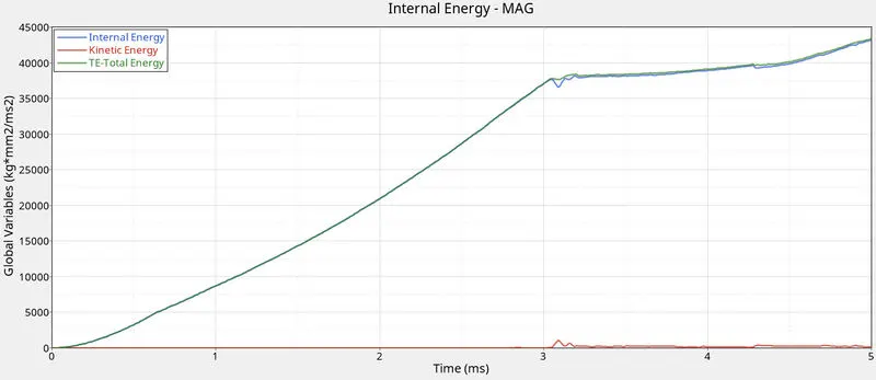
Based on energy graph, we can see that there is higher amount of internal energy in the model and when the elements in the model fail or break, the slope for internal energy and total energy bends towards x-axis but increases again at the end. This is the reason why we can see the PUNCH component getting displaced during the final stages of failure.

RESULTS :

Comparing all the seven cases, the Total number of cycles, Energy error, Mass error and Simulation time are entered in a tabulated format below.

CASE No.	Total number of cycles	Energy Error	Mass Error	Total Simulation Time (in seconds)
1	49380	-0.6% to 1.3%	0.00%	113.28
2	49217	-1.1% to 5.9%	0.00%	112.16
3	49408	-0.6% to 1.2%	0.00%	112.99
4	49304	-0.6% to 1.2%	0.00%	115.12
5	47969	-0.6% to 4.0%	0.00%	108.54
6	49508	-0.6% to 1.1%	0.00%	112.96
7	53202	-1.4% to 0.6%	0.00%	120.32

In Case 2, we can notice that the energy error is above 5% which states that the energy is generated due to the cracking of elements. In Case 7, we used LAW36 which accepts user defined function, so due to the complicated function defined in the model, it takes more number of cycles and thus more time than other cases to complete the simulation.

CONCLUSION :

We have basically used three different laws for this model. Although LAW2 and LAW27 both use Johnson-Cook to describe elasto-plastic behavior, they use different failure treatment. LAW2 checks with plastic strain and LAW27 checks with principal strain. Thus we get almost same results for both the laws.

LAW36 uses user defined functions where we can define a function consisting real life experimental data or lab data. So, the Case 7 or LAW36 (PLAS_TAB) would be the best to represent on field scenario as ultimately the material is going to follow the real time loading whereas simulation is only limited upto its own theory and imagination.