Proportional Valve simulation

Introduction: A safety relief valve is used to protect people, processes & properties. The protection is done by preventing overpressure in a process system by releasing a volume of fluid from the process when a predetermined maximum pressure is reached thereby reducing excess pressure.

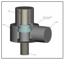
Overpressure: The maximum pressure in the system for which the spindle remains in its original position attached to the seat of the inlet is called the set pressure. When the inlet static pressure rises above the set pressure of the safety relief valve, the disc will begin to lift off its seat. As soon as the spindle starts to lift the spring compresses and the spring force increases. This means that the fluid pressure has to increase beyond the set pressure in order to lift the spindle further. The additional pressure rise, above the set pressure, is called the overpressure.

A wide range of different safety relief valves is available for many different applications and performance criteria. In our project, we are simulating the proportional valve. Proportional is the valve which

Objective: The main objective of this project is to run the simulations for two different cases, in order to determine the pressure force which is acting on the valve spindle at the different lifts.

Case 1: In this case, we have carried out a steady-state simulation with & without AMR for different valve lifts i.e for 3mm, 4mm & 5 mm

Case 2: In this case, we have carried out a Transient-state simulation with the FSI model without AMR in order to see valve dynamics as inlet pressure changes.

CASE 1

Geometry:

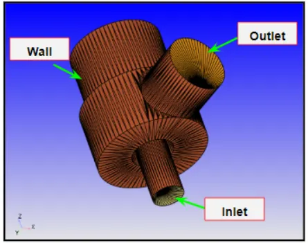
The pre-modeled geometry was imported into Converge and the geometry was inspected for surface error or other errors. After fixing all the errors & the boundaries were flagged & the case was set up.

Proportional valve

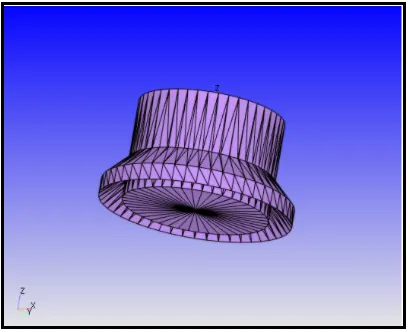
Valve-Spindle:

Case Setup:

• Application: General Flow
• Solver: Steady-state solver
• Simulation Type: Gas simulation
• Material: Air
• Species: N2=0.77 & O2=0.23
• Simulation mode: Full hydrodynamic

Simulation time parameters:

• Start time:0 cycle
• End time:15000 cycles

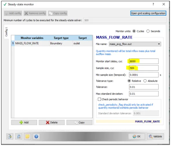
Steady-state Monitor: In Converge 3.0 we have an option for steady-monitor which basically monitors the results & stops the simulation once the results reach convergence.

In our case, we have enabled the steady-state monitor & we have used mass_flow_rate as monitor variable & we have given 8000 monitor start delay which means the Steady-state monitor will start to monitor the mass_flow_rate after 8000 cycles & also we have given 500 cycles sample size which means it will monitor the mass_flow_rate for 500 cycles & once the mass_flow_rate is same for continuous 500 cycles the converge will stop the simulation & we will achieve converged results.

Region & Initialization:

In this step, we have created a region of the fluid and initialize the pressure as 101325Pa & also the species value as N2=0.77 & O2=0.23

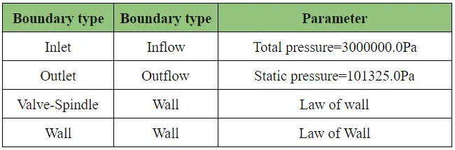
Boundary Conditions:

All the boundary conditions are defined at temperature=300K.

Physical Model

Turbulence model:k_e-epsilon

Grid Control:

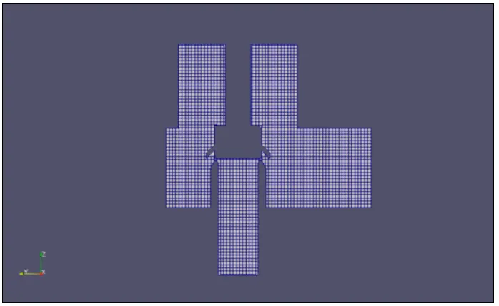
• Element size:dx = 0.004m, dy = 0.004m & dz = 0.004m

AMR

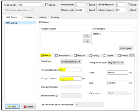
It’s essential to capture the data accurately were the shock occurs,so for this, we need more refine mesh or local mesh in that area while keeping the mesh size in the other area as same as the base grid size so, in order to do this we are using Adaptive mesh refinement technique.

In converge, adaptive mesh refinement gives a variety of based techniques in our case we will use velocity-based sub-grid-criterion with two-layer. Converge will monitors the curvature of velocity property provided in the AMR and refines the mesh when the property of velocity curvature between the consecutive grid is more than the defined SGS value.

AMR use the below formula to determine the refine grid size:

Refined mesh size=`frac{Base grid}{2^(MaxembeddLevel)}`

Output Files:

• The time interval for writing 3D output data files: 100 cycles (So, that we get at least 100 3D output files)
• The time interval for writing text output:1e-6 sec(So, that we get every minute )
• The time interval for writing restarting output:100 cycles
• Maximum number of restart file saved:3

Post-Processing

Mesh

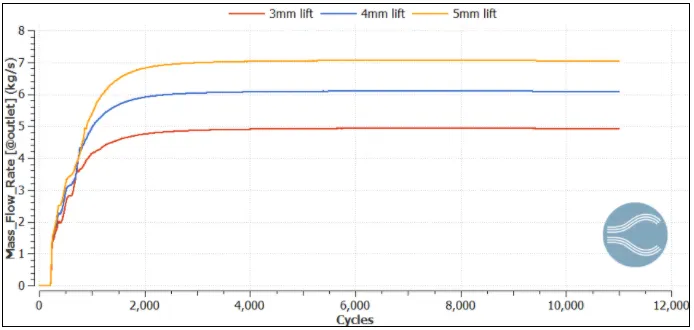
Mass flow rate plot

Without AMR

With AMR

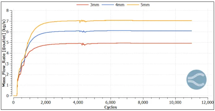
From the above plot, we can see that as lift increase the mass flow rate increase which is obvious as more lift means more space for fluid.

Velocity plot

Without AMR

With AMR

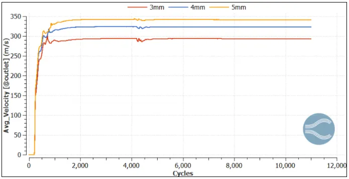
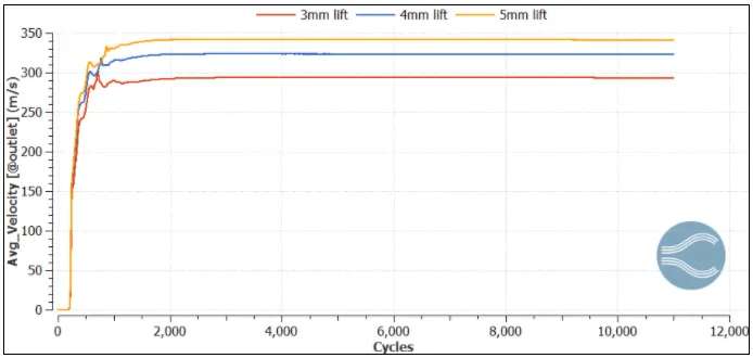
From the above plot, we can see that as lift increases the velocity increase which is obvious as more lift means more space for fluid, or in other words, we can say less obstructing area.

Pressure plot

Without AMR

With AMR

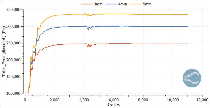
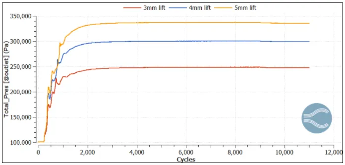
From the above plot, we can see that as lift increases the Total pressure increases which is because of velocity increase as we know total pressure is nothing but the summation of static plus dynamic pressure and at the outlet, we defined the static pressure which means it will remain constant & dynamic pressure will increase with a velocity which eventually increases the total pressure.

Pressure force plot

Without AMR

With AMR

Pressure force in z direction

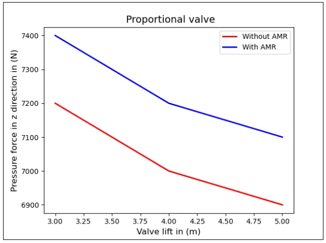
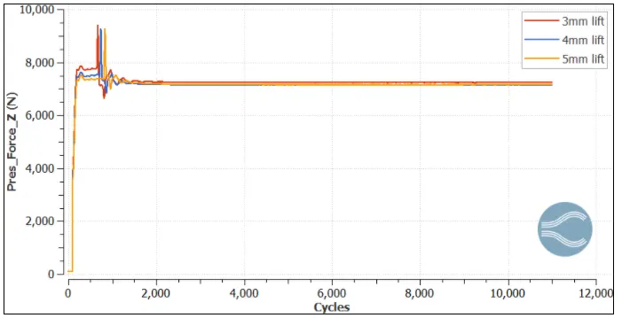
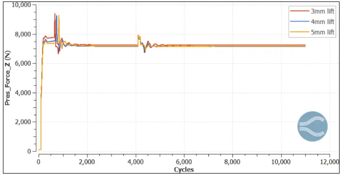
From the above plot, we can see that as lift increases the pressure force decreases which is obvious as more lift means more space for fluid to flow, or in other words, we can say that the fluid is pushing less to the valve spindle & because of this the pressure force decrease with increase in valve lift.

Comparison of without & with AMR

When we compare the result of mass flow rate, velocity, pressure force & total pressure without & with AMR though we have the same value this because of the SGS value which we have used in AMR but with AMR we are getting an actual physics flow because as we know the more we refined the mesh the more accurate results we get.

Contour:

Pressure contour for 3mm lift without & with AMR

Pressure contour for 4mm lift without & with AMR

Pressure contour for 5mm lift without & with AMR

Case 2

In this case, we have carried out a Transient-state simulation with the FSI model & without AMR in order to see valve dynamics as inlet pressure changes.

The geometry part of this case is similar to the above case.

Case Setup:

• Application: General Flow
• Solver: Transient solver
• Simulation Type: Gas simulation
• Material: Air
• Species: N2=0.77 & O2=0.23
• Simulation mode: Full hydrodynamic

Simulation time parameters:

• Start time:0 cycle
• End time:1.6 sec

Region & Initialization:

In this step, we have created a region of the fluid and initialize the pressure as 101325Pa & also the species value as N2=0.77 & O2=0.23

Boundary Conditions:

All the boundary conditions are defined at temperature=300K.

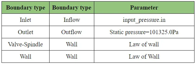
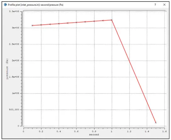
Intake pressure profile:

Physical Model

Turbulence model:k_e-epsilon

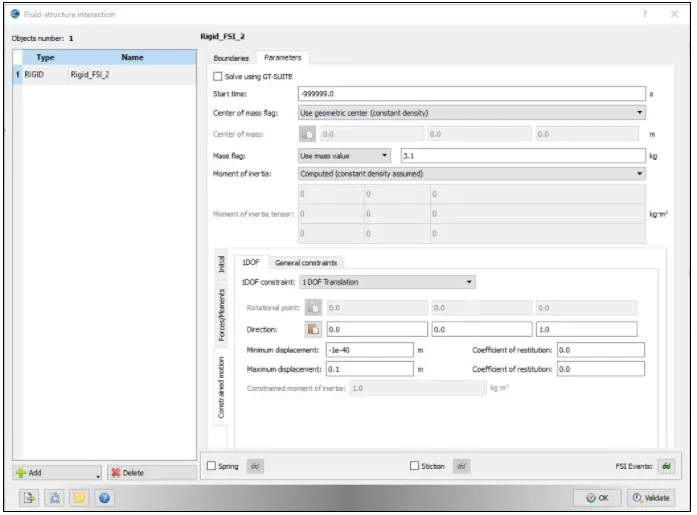
FSI model:

The interaction between the fluids & the solids is the phenomenon that can be seen in nature, for example, the deformation of trees caused by wind.

In almost the same manner the fluid will interact with the valve spindle & exerted the pressure force on the valve spindle that can lead to deformations. These deformations can be quite large or very small, depending on the pressure and velocity of the fluid and the material properties of the valve spindle. In order to simulate such flows, a Fluid-structure interaction modeling is used which is the subset of multiphase modeling.

Grid Control:

• Element size:dx = 0.004m, dy = 0.004m & dz = 0.004m

Output Files:

• The time interval for writing 3D output data files: 100 cycles (So, that we get at least 100 3D output files)
• The time interval for writing text output:1e-6 sec(So, that we get every minute )
• The time interval for writing restarting output:100 cycles
• Maximum number of restart file saved:3

Mesh plot:

Mesh animation:

Position plot

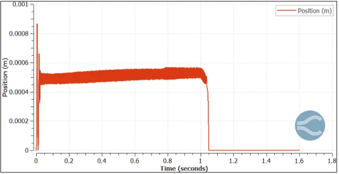
From the above plot, we can see the alternating nature of the valve spindle meaning the spindle is moving up & down & this happening because when the spindle valve moves its basic relief the pressure & because of this the pressure reduce up to a point were the spring force & mass of the valve dominates which basically pushing the valve back to his position. Also, we can see that amplitude of the valve spindle increase with respect to time but after one second the pressure get reduce to his initial pressure & the valve spindle back to his original position & this sudden drop in pressure is because the pressure profile which we have given at the inlet.

Force acting on valve spindle:

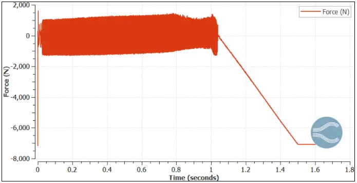
From the above plot, we can see that the initial force acting on the valve spindle is around 7000 (negative sign indicates the opposite direction) which is basically keeping the valve closed & also we can see the fluid is imparting more than 7000N force on the valve spindle in order to open it & after that, the force gets fluctuate till pressure get restore to its the initial value and once get restored the force get back to his baseline value & valve gets closed.

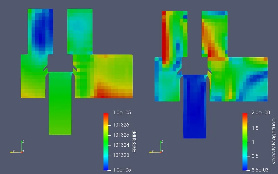
Contour:

Conclusion:

Successfully simulated the proportional valve case with & without AMR also we did FSI simulation on proportional valve.