open_system('spe_servomotor/DC Servo Motor')

The DC motor model shows a relationship from current to torque (the green line on the left). The torque causes the shaft of the motor to spin and we have a relationship between this spinning to the Back EMF (electromotive force). The rest of the parameters include a shaft inertia, viscous friction (damping), armature resistance, and armature inductance.

While manufacturers may provide values for some of these quantities, they are only approximate. We want to estimate these parameters as precisely as possible for our model to ascertain whether it is an accurate representation of the actual DC servo motor system.

Key highlights:-

Mathematical modeling from the first principles:-

Get Started

Learn the basics of System Identification Toolbox

Data Preparation

Plot, analyze, detrend, and filter time- and frequency-domain data, generate and import data

Linear Model Identification

Identify impulse-response, frequency-response, and parametric models, such as state-space and transfer function models

Nonlinear Model Identification

Identify nonlinear ARX, Hammerstein-Wiener, and grey-box models

Grey-Box Model Estimation

Estimate coefficients of linear and nonlinear differential, difference and state-space equations

Model Validation

Compare model to measured output, residual analysis, response plots with confidence bounds

Model Analysis

Discretize models, convert models to other types, linearize nonlinear models, simulate and predict output

Time Series Analysis

Analyze time series data by identifying linear and nonlinear models such as AR, ARMA, state-space, and grey-box models, performing spectral analysis, and forecasting model outputs

Online Estimation

Estimate model parameters and states during system operation, generate code and deploy to embedded targets

Modeling on electrical engineering system:-

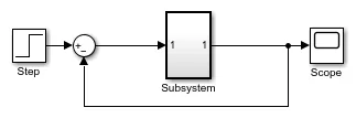
In a Simulink^® model, an algebraic loop occurs when a signal loop exists with only direct feedthrough blocks within the loop. Direct feedthrough means that Simulink needs the value of the block’s input signal to compute its output at the current time step. Such a signal loop creates a circular dependency of block outputs and inputs in the same time-step. This results in an algebraic equation that needs solving at each time-step, adding computational cost to the simulation.

The model in the figure is equivalent to this system of equations in semi-explicit form:

The system has neither algebraic variables nor direct feedthrough and does not contain an algebraic loop.

Modify the model as described in the following steps:

Simulink based modeling:-

Main Content

Modeling

Design models of dynamic systems

Use Simulink^® to model algorithms and physical systems using block diagrams. You can model linear and nonlinear systems, factoring in real-world phenomena such as friction, gear slippage, and hard stops.

To show the first stage of a modeling workflow that begins with limited information, this example uses a simple mechanical system composed of a mass, spring, and damper.

This second-order differential equation characterizes the system:

where

• is mass

• is the damping coefficient

• is the spring constant

• is acceleration

• is velocity

• is displacement

• is force

Solving for provides a form of this equation that maps more clearly to a Simulink® model.

In model ex_modeling_simple_system, a Sum block computes the forces applied to the mass, the Gain block labeled 1/m computes the acceleration of the mass, and the Second-Order Integrator block solves for the velocity and position of the mass.

Control law design and test:-

Notice that units are visible on the model and subsystem icons and signal lines. Units are specified on the ports and on the bus object.

To open the control_logic Stateflow chart, double-click on it in the fuel_rate_control subsystem.

Dynamic system

[x,u,y,dx] = trim('sys')
[x,u,y,dx] = trim('sys',x0,u0,y0)
[x,u,y,dx] = trim('sys',x0,u0,y0,ix,iu,iy)
[x,u,y,dx] = trim('sys',x0,u0,y0,ix,iu,iy,dx0,idx)
[x,u,y,dx,options] = trim('sys',x0,u0,y0,ix,iu,iy,dx0,idx,options)
[x,u,y,dx,options] = trim('sys',x0,u0,y0,ix,iu,iy,dx0,idx

,[x,u,y,dx,options] = trim('sys',x0,u0,y0,ix,iu,iy,dx0,idx,options,t) sets the time to t if the system is dependent on time.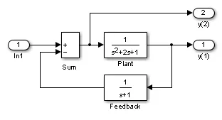

matlab script to define modeling and control design parameters

D — Control signal for scheduling periodic events
scalar

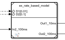
Periodic event ports provide function-call control signals that specify when to execute the model. For an example, see Test Rate-Based Model Simulation Using Function-Call Generators.

Each port label displays information about the periodic event, such as the sample time of the corresponding Inport block. For example, the Model block in this image displays periodic event ports and references a model with two discrete rates: 0.01 and 0.1.

Dependencies

To enable this type of port, set Schedule rates with to Ports.

Open this model to see a simple counter. The model counts up from zero to a threshold value and then wraps back to zero. The threshold value is set to 15. To change the threshold value, change the value of the input to the count_threshold port. The Enable signal specifies whether the counter counts upward or holds the previous value. A value of 1 indicates that the counter counts upward continuously.

Verification Methods

If you have HDL Verifier™ installed, you can also verify the generated HDL code by using these methods.

Verification Method
HDL Cosimulation
SystemVerilog DPI Test Bench
FPGA-in-the-Loop

In this tutorial, we will consider the following unity-feedback system:

The output of a PID controller, which is equal to the control input to the plant, is calculated in the time domain from the feedback error as follows:

(1)

First, let's take a look at how the PID controller works in a closed-loop system using the schematic shown above. The variable () represents the tracking error, the difference between the desired output () and the actual output (). This error signal () is fed to the PID controller, and the controller computes both the derivative and the integral of this error signal with respect to time. The control signal () to the plant is equal to the proportional gain () times the magnitude of the error plus the integral gain () times the integral of the error plus the derivative gain () times the derivative of the error.

This control signal () is fed to the plant and the new output () is obtained. The new output () is then fed back and compared to the reference to find the new error signal (). The controller takes this new error signal and computes an update of the control input. This process continues while the controller is in effect.

The transfer function of a PID controller is found by taking the Laplace transform of Equation (1).

(2)

where = proportional gain, = integral gain, and = derivative gain.

We can define a PID controller in MATLAB using a transfer function model directly, for example:

Kp = 1;
Ki = 1;
Kd = 1;

s = tf('s');
C = Kp + Ki/s + Kd*s

C =
 
  s^2 + s + 1
  -----------
       s
 
Continuous-time transfer function.

Suppose we have a simple mass-spring-damper system.

The governing equation of this system is

(3)

Taking the Laplace transform of the governing equation, we get

(4)

The transfer function between the input force and the output displacement then becomes

(5)

Let

    m = 1 kg
    b = 10 N s/m
    k = 20 N/m
    F = 1 N

Substituting these values into the above transfer function

(6)

The goal of this problem is to show how each of the terms, , , and , contributes to obtaining the common goals of:

• Fast rise time
• Minimal overshoot
• Zero steady-state error

• Let's first view the open-loop step response. Create a new m-file and run the following code:

  s = tf('s');
  P = 1/(s^2 + 10*s + 20);
  step(P)
  

  The DC gain of the plant transfer function is 1/20, so 0.05 is the final value of the output to a unit step input. This corresponds to a steady-state error of 0.95, which is quite large. Furthermore, the rise time is about one second, and the settling time is about 1.5 seconds. Let's design a controller that will reduce the rise time, reduce the settling time, and eliminate the steady-state error

• Let the proportional gain () equal 300 and change the m-file to the following:

  Kp = 300;
  C = pid(Kp)
  T = feedback(C*P,1)
  
  t = 0:0.01:2;
  step(T,t)
  

  C =
   
    Kp = 300
   
  P-only controller.
  
  
  T =
   
          300
    ----------------
    s^2 + 10 s + 320
   
  Continuous-time transfer function.