Project - Position control of mass spring damper system
Given Data:-
m = 3.6 kg
k = 400 N/m
c = 100Ns/m
Transfer function for a spring mass damper system is 1/(m*s^2+c*s+k)
where m is mass, c is damping coefficient and k is spring constant.
after subtituting the respective values in the transfer function
1/(3.6*s^2+100*s+400)
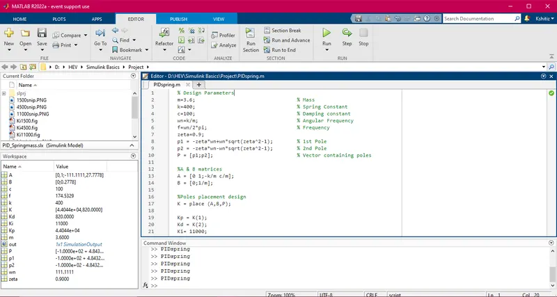
% Design Parameters
m=3.6; % Mass
k=400; % Spring Constant
c=100; % Damping constant
wn=k/m; % Angular Frequency
f=wn/2*pi; % Frequency
zeta=0.9;
p1 = -zeta*wn+wn*sqrt(zeta^2-1); % 1st Pole
p2 = -zeta*wn-wn*sqrt(zeta^2-1); % 2nd Pole
P = [p1;p2]; % Vector containing poles
% A & B matrices
A = [0 1;-k/m c/m];
B = [0;1/m];
% Poles placement design
K = place (A,B,P);
Kp = K(1);
Kd = K(2);
Ki= 11000;
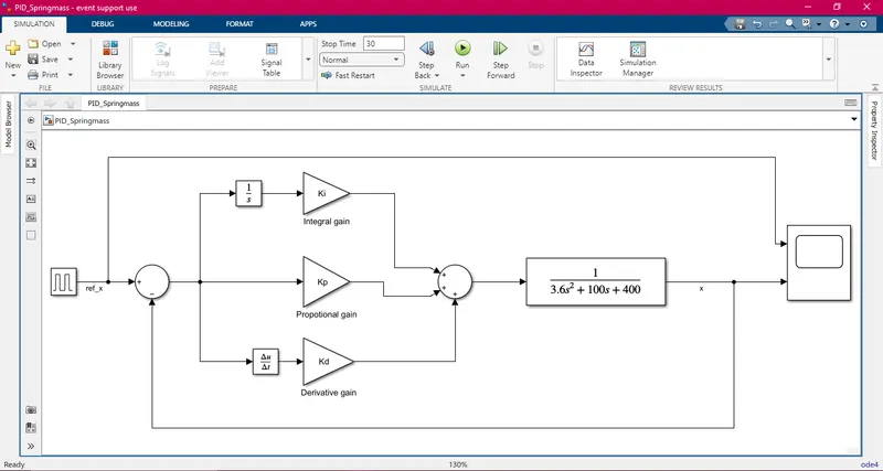
In this model, we have used a Pulse generator as the reference signal. Two mathematical operators blocks are used to conduct mathematical operations. Three gain blocks are used for the Integral(Ki), Proportional(Kp) and Derivative gains(Kd) respectively. One integrator block is used to integrate the signal and one derivative block is used to differentiate the signal. A transfer function is used to function as the spring mass damper system with respective co-efficients. This makes the model much clear. A scope block is used to plot the graph and analyse the results after simulation.
The below result has been shown after several trials of diffferent Ki values to obtain an error free result or minimum possible error state and hence to show the clarity in the stages and simulation, three different values of Ki has been picked to show the arrival of the optimum value.
Case: 1
When Ki= 1500
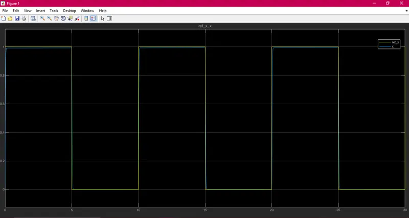
We can clearly see that when the value is kept at 1500 the scope shows steady state error after the simulation. The x (blue) and x_ref (yellow) on different time stamps has slight error as the graph moves from 0 to 30.
Case: 2
When Ki=4500
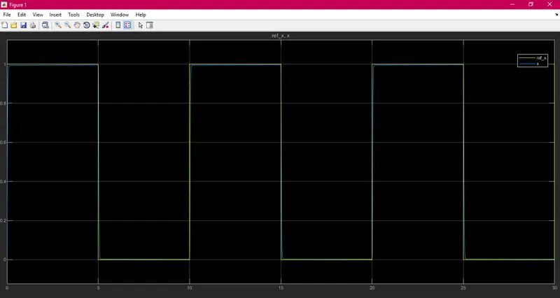
When we increased the value of Ki the result we can see is better than the previous simulation the error percentage has decreased significantly but we can still see slight error and scope of improvement in the performance after the simulation.
Case: 3
When Ki=11000
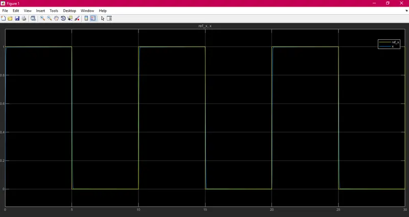
When Ki is kept above 10000 or as in this case 11000 we can see a drastic improvement from the 1st case where the steady state error has decreased drastically.
We can see that by increasing the value of Ki we can decrease the steady state error.