Project - Data Handling and Interpolation

Final Project

Matlab code for interpolation

close all ; clear all; clc;

% interpolation of voltge And current data
A = xlsread('VI.xlsx');  %reading excel file data 
x = A(:,1);  %voltage data seperating 
y = A(:,2);  %current data seperating 
xq = [-17.3:0.1:0.9];  %interpolation range
yq1 = interp1(x, y, xq)  %linear interpolation
yq2 = interp1(x, y, xq,'spline'); %spline interlopation
figure(1)
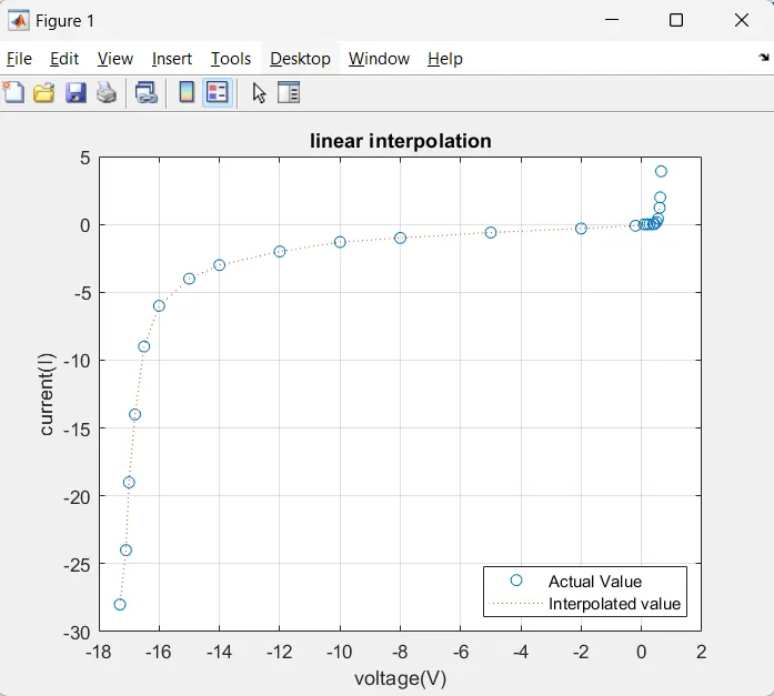
plot(x, y,'o', xq, yq1,':');   %plot for linear interpolation 
title('linear interpolation'); %plot title name
xlabel('voltage(V)'); % label for x
ylabel('current(I)');  % label for y
legend('Actual Value', 'Interpolated value', 'location','southeast');  % legend for better understanding
grid on
figure(2)
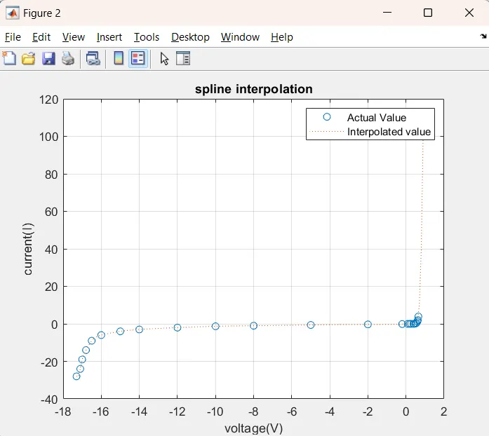
plot (x, y, 'o', xq, yq2,':'); % plot for spline interpolation   
title('spline interpolation' );% naming the plot to make diffrence between both plots 
xlabel('voltage(V)'); % label for x
ylabel('current(I)'); % label for y
legend('Actual Value', 'Interpolated value', 'location','Northeast');  % legend for better understanding
grid on
% saving interpolation data in text file
data_handle = fopen('data_file.txt','w'); % initialising name of text file which we have to write
fprintf(data_handle, '%4.4f %3.3f \n', yq1, yq2);% printing the values
fclose(data_handle)

Result

Plot for linear interpolation

Plot for spline interpolation

M-script explanation

Firstly, clearing the ‘workspace’ memory by giving the ‘clear’ command.

To clear the command window, we used the ‘clc’ command. Then given input excel data file is read by using the ‘xlsread’ function command. The input values of Voltage and current are separated by using this syntax (:,1) and (:,2). The interpolation range is defined as per the given in the project description.

The linear interpolation is calculated by using this syntax – Interp1(); in this calculation, we used the voltage and current data.

For spline interpolation, we use the syntax – Interp1(); and mention the spline. To calculate the spline interpolation. After performing the interpolation, the plot is plotted. To view the plot we use the figure (1) command.

The linear interpolation is plotted using the figure (1) command and plot command by providing the actual values of voltage v and current i and the 's' specified square shape of the marker. And the interpolation of the voltage and current is also drawn in the same plot by using xq and yq1 with an indication of ‘.’

X and Y labels are used to label the x and y-axis. After that for the title of the graph ‘title ()’ command is used. Then for the legend, we used legend () syntax. In legend syntax, we are using actual values, interpolated values, markers, and line styles. The legend is placed at the northeast of the graph. Then for the grid lines in the graph, we used the “grid” command.

For saving the output data into a text file is created with the name ‘VI_output.txt’ for this we used the command 'fopen ()’. Then the interpolated and spline values are saved by using the ‘fprintf ()’ command.