Project - Data Handling and Interpolation

Answer :-

Interpolation - In engineering or some application, we can into situations where some data might not be available. Interpolation is a technique for adding new data points within a range of a set of known data points. You can use interpolation to fill-in missing data, smooth existing data, make predictions, and more.

Types of interpolation methods are:

1. Linear interpolation
2. Nearest neighbor interpolation or Piecewise constant interpolation
3. Polynomial interpolation
4. Spline interpolation
5. Mimetic interpolation
6. Cubic Spline Interpolation

Matlab lncludes - For curve data, you can set Interpolation method to Linear , Nearest neighbor , Cubic Spline , or Spline . For surface data, you can set Interpolation method to Nearest neighbor , Linear , Cubic Spline , Biharmonic (v4) , or Thin-plate spline.

Interpolation Functions in MaTlab -

The interp family of functions includes interp1, interp2, interp3, and interpn. Each function is designed to interpolate data with a specific number of dimensions. interp2 and interp3 use grids in meshgrid format, while interpn uses grids in ndgrid format.

The below code can be refer for the ask question -

VI=xlsread("VI.xlsx"); %reading given excel sheet
V=VI(:,1); % reading voltage value
I=VI(:,2); % reading current value
xq = -17.3:0.1:0.9; % defining the range for interpolation
yq1 = interp1(V,I,xq); % applying interpolation
figure(1);
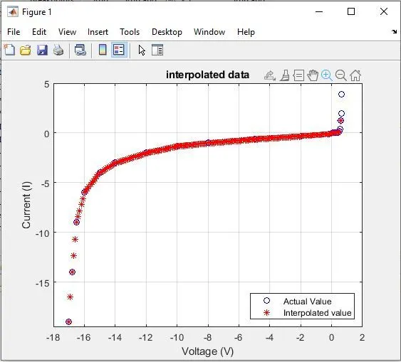
plot(V,I,'bo',xq,yq1,'r*'); % plotting the interpolation
title('interpolated data');
xlabel('Voltage (V)'); % annotation
ylabel('Current (I)');
legend({'Actual Value', 'Interpolated value'},'Location','southeast');
grid;

fileID = fopen('interpolated_data.txt','w'); % creating and saving the file
fprintf(fileID,'%8s %10s\n','volt','current');
fprintf(fileID,'%f %f\n',yq1);
fclose(fileID);

Graph plotted from the above code is shown below -

M file of above code and Interpolated data text file is attatched below.