Project - Data Handling and Interpolation

>> Q project on interpolation :

data = readmatrix('VI.xlsx'); % opening and getting data from table

V=data(:,1); % getting data from column 1 for voltage

I=data(:,2); % getting data from column 2 for current

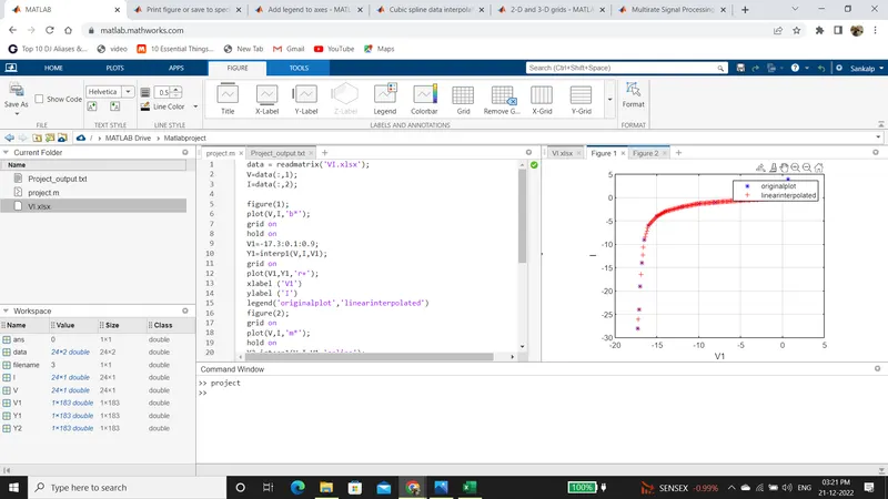
figure(1); %ploting the intial data fig.

plot(V,I,'b*');

grid on

hold on

V1=-17.3:0.1:0.9; % assiging the given range

Y1=interp1(V,I,V1); % using interpolation to plot between original values

grid on

plot(V1,Y1,'r+'); % ploting the interpolated graph for linear interpolation

xlabel ('V1')

ylabel ('I')

legend('originalplot','linearinterpolated')

figure(2); % ploting the original fig, for spline interpolation

grid on

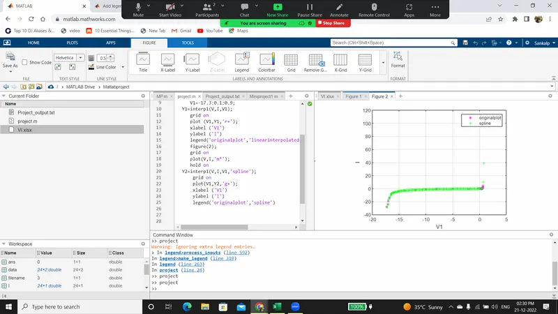
plot(V,I,'m*');

hold on

Y2=interp1(V,I,V1,'spline'); % using spline interpolation

grid on

plot(V1,Y2,'g+'); % ploting spline interpolation

xlabel ('V1')

ylabel ('I')

legend('originalplot','spline')

% writing the project.m to an output file called Project_output.txt

filename=fopen ('Project_output.txt','w');

fprintf(filename,'%d t', Y1,Y2);

fclose(filename);

>> observation

with help of this program, we plotted a graph of the VI curve for discrete values, and with the help of interpolation, we also plotted for data between these discrete points. we are doing interpolation to find the missing data, interpolation can be in 1D or can be in 2D . here in these example we have identified the missing data which are attached as a text file.

figure 1 gives us a 'linear interpolation', through observation we notice that the curve is not very smooth and is linear in nature.

figure 2 gives us a 'spline interpolation', through observation we can notice that the curve is a very smooth one and is much more decent than the linear interpolation figure.