Project

Aim:-

Preparing the model of the vehicle containing all basic system-level components of the all-terrain vehicle(ATV).

Objective:-

1. Analyzing and describing the parameters of the physical system blocks used in building the model in Simulink.
2. Describing the connections between the systems.
3. Analyzing all the results obtained after the simulation.

Theory:-

What is ATV?

An all-terrain vehicle (ATV), also known as a light utility vehicle (LUV), a quad bike, or simply a quad, as defined by the American National Standard Institute (ANSI); is a vehicle that travels on low-pressure tires, with a seat that is straddled by the operator, along with handlebars for steering control. As the name implies, it is designed to handle a wider variety of terrain than most other vehicles.

Major Components used in building the model in Simulink:

Generic Engine, Continuously Variable Transmission(CVT), Simple Gear, Vehicle body, Tire, Ideal Rotational Sensor, Double Shoe Brake, Inertia Source, Signal Builder, Lookup Table, Constant Block, Step, Knob, Full Guage, Solver.

Model prepared for the study and simulation of the ATV are of four types out of which the first two are without a lookup table and among these two one has an input to the generic engine through the signal builder and the other uses manual input using knobs. And in the other two models where the lookup table is used for the input signal to the CVT one of them uses a step block and the other uses the manual input using a knob.

Description of the common components in all four models:

Generic Engine:

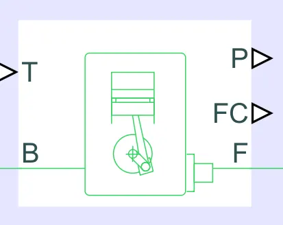
The generic engine block represents the basic form of SI/CI engines and as shown in the figure it contains 5 ports.

Port T in the figure represents the throttle input provided to the engine. In the models, the throttle input is provided in various forms i.e. through a signal builder or through the knobs via a constant block, or through a step signal.

B and F ports are the mechanical rotational conservation ports where B represents the engine block and F represents the crankshaft of the engine.

P and FC ports are the output signal ports representing power and fuel consumption respectively.

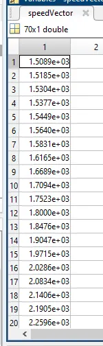
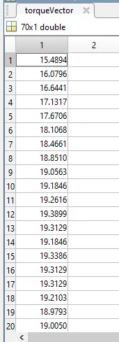
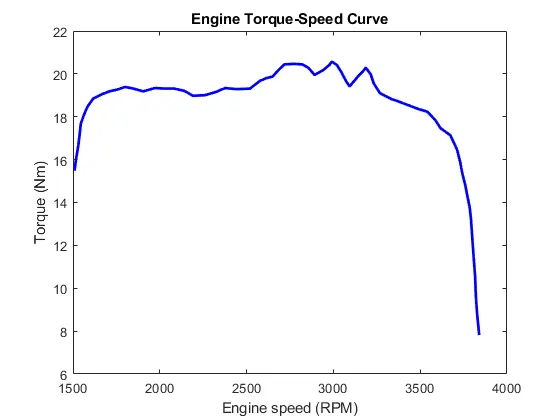
And the parameters mentioned in the block are speed vector, torque vector, engine inertia, initial velocity, and speed threshold it is the threshold below which the engine will be stalled and torque will be rendered to zero. Speed and Torque in parameters are the arrays of 70 data points as shown in the figure below the plot of the speed vector vs torque vector is also provided below.

Continuously Variable Transmission(CVT):

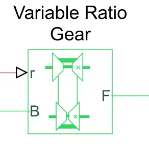
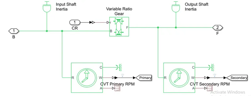
As shown in the figure above the variable ration gear block given over here represents the physical CVT system which changes the gear ratio continuously according to the velocity and torque from the input shaft and load on the output shaft.

Over here the port R represents the input signal for the ratio of the gear connected between the input and output shaft for the input signal first two models without a lookup table use the signal builder and the other two models use the lookup table to vary the ratio of the transmission between and output shaft.

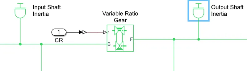
Port B and F represent the mechanical rotational conservation here port B is connected to the input shaft and port F is connected to the output shaft. An inertia source is also connected as shown in the figure below and in the parameter part of the inertia source equations m1*(((18.6e-2)/2)^2+((2.5e-2)/2)^2)/2 and m2*(((19.8e-2)/2)^2+((1.9e-2)/2)^2)/2 are used where m1 = 3.5 and m2 = 3.2 here the equation are obtained according to the geometry of the shafts.

Ideal Rotational Sensor:

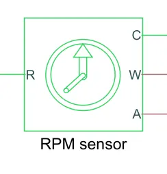
The ideal rotational sensor is shown in the figure above senses the rotational motion of various parts and provides data on angular velocity and angular displacement.

Ports W and A in the sensor are for the output signal of the angular velocity and angular displacement respectively.

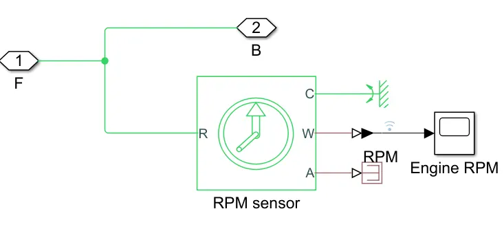
Ports R and C are mechanical rotational conservation ports, in the three rotational sensors are used first one for sensing the output angular velocity of the engine crankshaft, and the second and third sensors are used for sensing the angular velocity of input and output shaft of the CVT. All three sensor connections are shown in the figure below

Vehicle Body:

The vehicle body in the Simulink model represents the common vehicle body for all types of vehicles.

Parameters of the vehicle body are as follows:

• Mass of the vehicle is 250 kg.
• No. of the wheels per axel in the model is 2.
• Horizontal distance between the Front axel and Center of Gravity(CG) is 1 m.
• Horizontal distance between the rear axel and CG is 0.35 m.
• Height of CG above the ground is 0.7 m
• Gravitational accelaration is 9.81 m/s^2.
• Frontal area 0.735482 m^2
• Drag coefficient is 1.92
• Air density is 1.18 kg/m^3.
• Initial velocity is 0 m/sec.

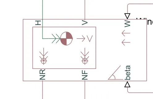
As shown in the figure above the vehicle body has 8 ports with 2 ports being optional.

Port H is the mechanical translational conserving port associated with the horizontal motion of the vehicle body. The resulting traction motion developed by tires should be connected to this port. It is an input port of the vehicle body.

Port V is for the output signal of the velocity of the vehicle and an integrator block is also attached to the velocity signal to obtain the displacement of the vehicle.

Ports NR and NF are the output signal of the normal forces acting on the rear and front axle wheels and it is considered positive when it is acting in the downward direction.

Ports W and beta are the input signal ports for the headwind speed acting on the vehicle body and the inclination of the vehicle on which the vehicle is running respectively ports

Ports CG and M are the optional ports that are exposed when we need to add the additional mass to the vehicle body they are input values of the CG distance and the value of the additional mass.

Tire (Magic Formula):

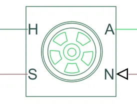
Tire (magic formula) is the model of the physical tire which uses the magic formula for the calculation of all the forces and slip acting on the tire while it is interacting with the road.

Parameters of this model can be provided in 4 different ways as follows:

• Peak longitudinal force and corresponding slip
• Constant magic formula coefficients
• Load dependent magic formula coefficients
• Physical signal magic formula coefficients

In the model, the parameters are entered using the Peak longitudinal force and corresponding slip option and the parameters entered are:

• Rated vertical load = 2060 N
• Peak longitudinal force at rated load = 1260 N
• Slip at peak force at rated load = 5
• Rolling radius = 0.2921 m
• Tire inertia = 0.01 kg*m^s
• Initial velocity = 0 rpm
• Rolling resistance constant coefficient = 0.015
• velocity threshold = 0.1 m/s

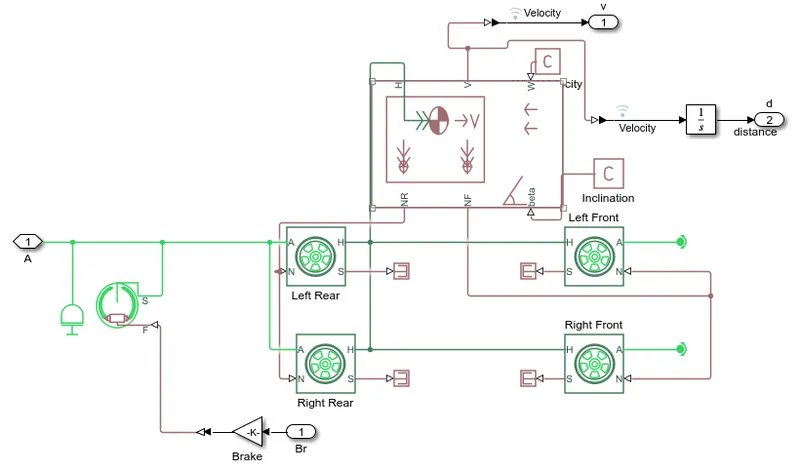
As shown in the figure the tire model contains 4 ports of which port H is for the horizontal translational motion conserving port of the wheel which outputs the signal of the thrust developed by the tires to the vehicle body and is connected to the vehicle body and other axels wheel as shown in the figure below.

Port N is the normal force acting on the tire from the vehicle body it is the input signal of the tire connected to the output signal of the normal force port of the vehicle body as shown in the figure below.

Port S is the output signal port reporting the tire slip data.

Port A is the mechanical rotational conserving port and this port of the rear tire is connected to the input velocity signal from the simple gear of the model for rotational force to act on the wheel, inertia source, and double shoe brake are attached to the incoming signal to provide the inertia and damping to the input shaft and the front wheels port is connected to the free rotational end which represents that the front wheels are freely rotated and driven.

Simple Gear:

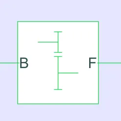
It is a simple gear with two ports B and F, in which B is connected to the output shaft of the CVT of the model and port F is connected to the input port of the rear wheels of the vehicle. In the parameters of the simple, the gear ratio of 10 is provided which is the ratio of F/B with no backlash and friction losses.

Double shoe brake:

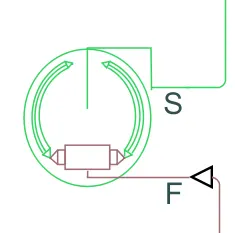
The double shoe brake block in the Simulink contains 2 ports S and F, where S is the mechanical rotational conserving port which represents the drum of the wheels of the vehicles and F is the input signal for the force provided to the brakes actuator it gets it input from the brake signal generated outside the subsystem.

Parameters entered in the double shoe brake are as follows:

• Drum Radius = 150 mm
• Actuator location radius = 100 mm
• Pin Location radius = 125 mm
• Pin location angle = 15 deg
• Shoe beginning angle = 5 deg
• Shoe span angle = 120 deg
• Viscous friction coefficient = 0.01 Nmsec/rad
• Constant friction coefficient = 0.3

Distinct features of each model :

1)ATV model without lookup table and fixed brake and throttle input signal to the engine

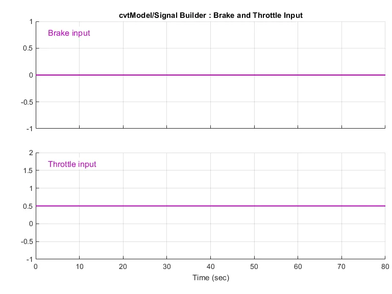
In this model, the input to the generic engine throttle is provided through the signal builder of the Simulink and the signal provided is as shown in the figure below. This signal builder also includes a signal for brake force which is an input force signal for double shoe brake which is connected to the vehicle's rear wheels.

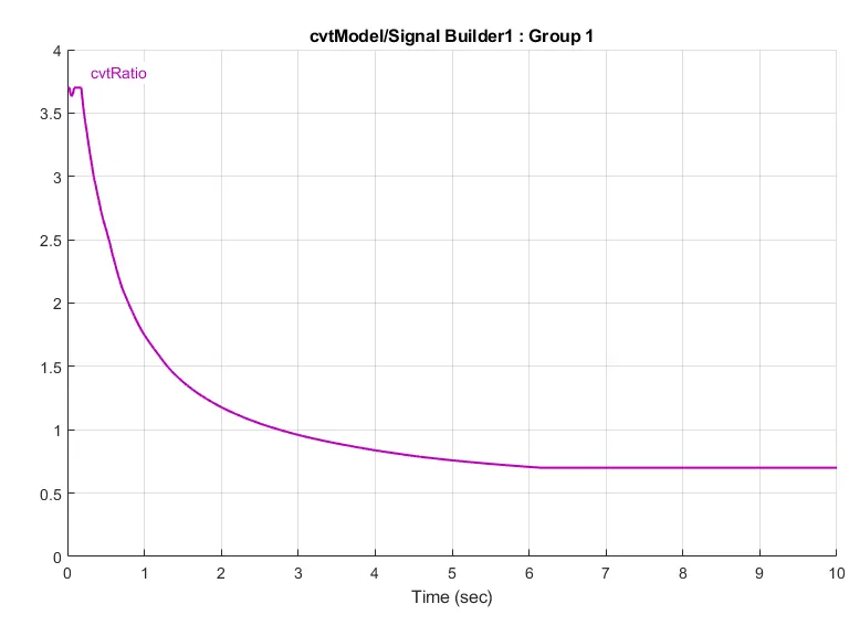
And the inputs provided to the CVT is also through the signal builder and input values during the simulation are shown in the plot below, CVT changes the ratio of the input to output shaft over time as shown in the plot below in which it initially fluctuates near 3.7 and then decreases exponentially up to 2.5 sec and then it settles at about 0.7 where it stabilizes and remains almost constant with time.

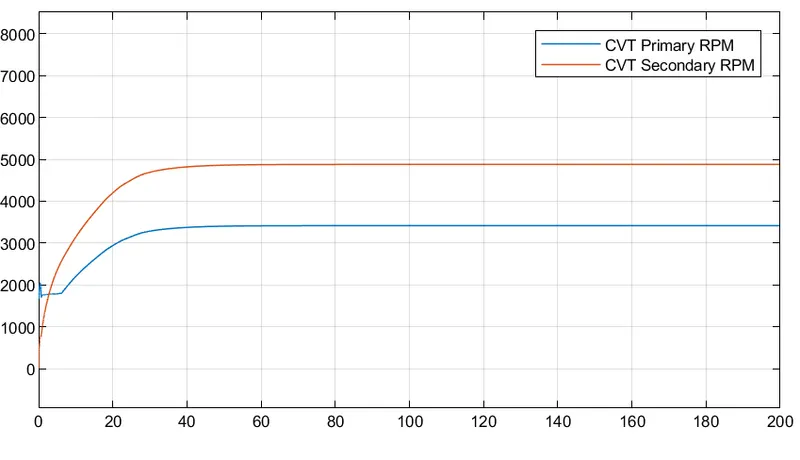
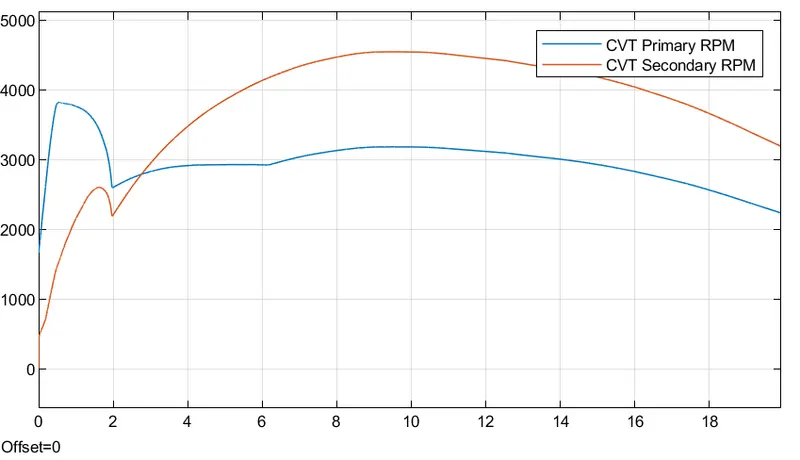
And the results of this variable on the input (Primary) and output (Secondary) shaft's angular velocity can be seen in the plot below, here it is seen that there is variation in the input shaft velocity due to variation in the CVT ratio but these sudden changes are damped in the output shaft due to the damping effect in the CVT gear and we get a jerk-free motion in the input of the simple gear. Here it can be seen that at about 2.7 sec the angular velocity of the output shaft is more than the input shaft as the ratio of the output to input becomes more than 1 at this time.

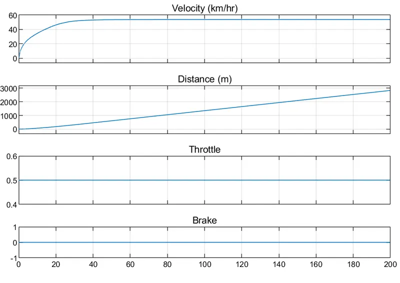
And the velocity and displacement of the vehicle when the throttle valve is kept fixed at 0.5 and the brake is not applied is given in the plot below, here in the plot it can be seen that the displacement of the vehicle is constantly increasing over time and velocity is initially increasing parabolically and then remains constant this is due to the inertia of the vehicle.

2) Model with varied throttle and brake input through the dashboard and without a lookup table.

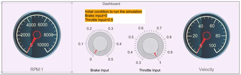
In this model, a dashboard containing the knobs to vary the input of the throttle and brake inputs to the engine is provided, as also full gauges to visualize the linear velocity of the vehicle and angular velocity of the crankshaft of the engine. As shown in the figures the knob signal is connected with the constant blocks which input the signal to the generic engines in the form of throttle and brake input to the double shoe brake connected to the rear wheels of the vehicle.

CVT ratio input signal graph is as same as the previous model in which it initially fluctuates near 3.7 and then decreases exponentially up to 2.5 sec and then it settles at about 0.7 where it stabilizes and remains almost constant with time.

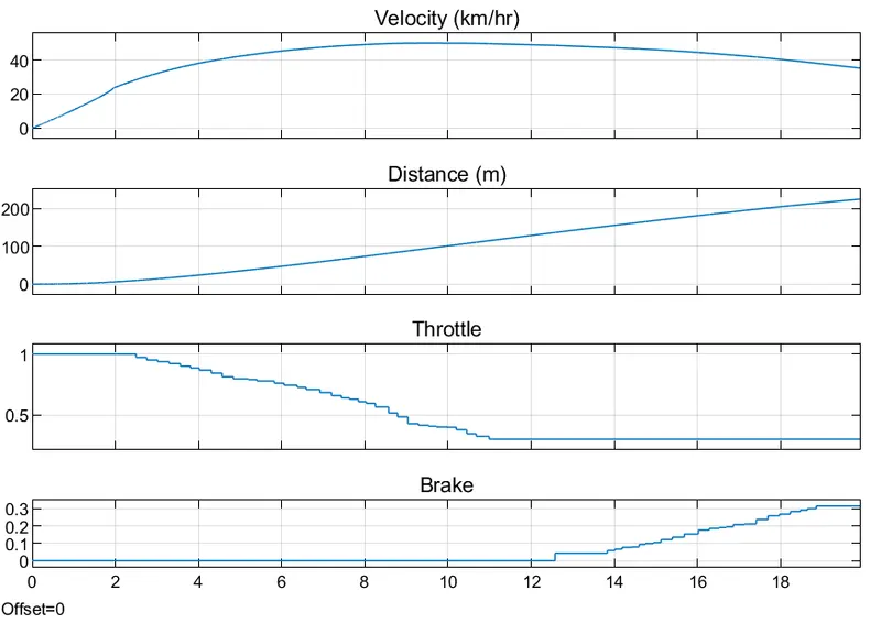
The figure provided below is the plot of the throttle and brake input over time and through it the plot of the velocity and displacement of the vehicle, and angular velocity of the input and output shaft would be deduced in the model the simulation run speed is paced at 1 sec to visualize the changes properly.

As is seen in the figure the velocity of the vehicle and displacement is changing according to the changes in the throttle and brake input values. Here the throttle is decreased gradually and brake force is increased gradually

And the results of this variable on the input (Primary) and output (Secondary) shaft's angular velocity can be seen in the plot below, here it is seen that there is variation in the input shaft velocity due to variation in the CVT ratio but these sudden changes are damped in the output shaft due to the damping effect in the CVT gear and we get a jerk-free motion in the input of the simple gear. Here it can be seen that at about 2.7 sec the angular velocity of the output shaft is more than the input shaft as the ratio of the output to input becomes more than 1 at this time.

3) Model with the lookup table and without the dashboard.

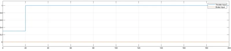
In this model the input of the throttle to the generic engine and brake force to the double shoe brake is in the form of the step here the value of the throttle is kept at 0.3 for 20 secs and then the throttle valve is fully opened for the rest of the simulation and the brake force provided is null. The plot of the throttle and brake is given below.

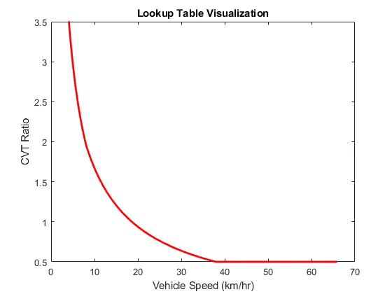
And lookup table is used to adjust the ratio of the CVT according to the speed of the vehicle and the plot of the Speed vs CVT ratio is given below in this it can be seen that the CVT ratio is 3.5 for the max. torque generation at the 0 to 5 kmph initial velocity and then it is reduced exponentially to 0.5 when the speed reaches about 37 kmph.

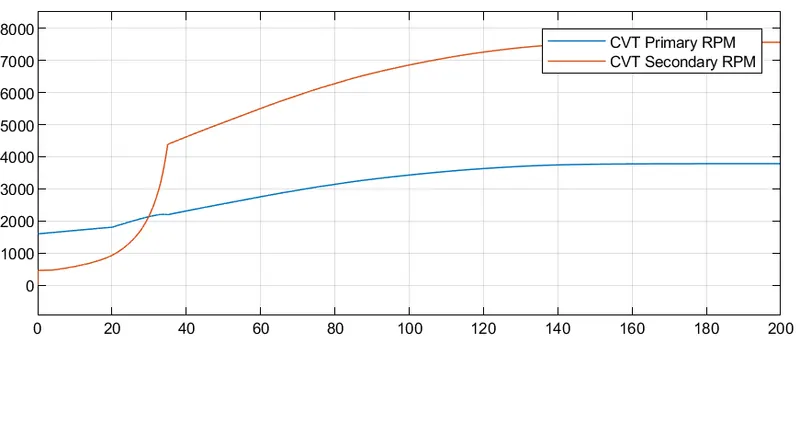
And the plot of the time vs angular velocity of the input(Primary) and output(Secondary) shaft is given below. Here it can be seen that at about 30 sec the velocity of the vehicle is more than 20 kmph the angular velocity of the output shaft is more than the input shaft as the ratio of the output to input becomes more than 1. And the sudden change in the velocity represents the ratio stabilizing suddenly at 0.5 when the linear velocity of the vehicle reaches about 38 kmph.

The plot of the comparison of the linear velocity to the throttle value and brake force is given below where it can be seen that the linear velocity of the vehicle starts increasing exponentially at about 20 secs which when the throttle valve is fully opened and then it suddenly stabilizes which the point where the CVT ratio settles to 0.5.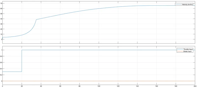

4) Model with lookup table and dashboard.

In this model, a dashboard containing the knobs to vary the input of the throttle and brake inputs to the engine is provided, as also full gauges to visualize the linear velocity of the vehicle and angular velocity of the crankshaft of the engine. As shown in the figures the knob signal is connected with the constant blocks which input the signal to the generic engines in the form of throttle and brake input to the double shoe brake connected to the rear wheels of the vehicle.

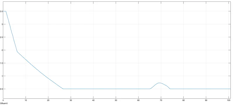
In this model, the lookup table used is the same as the previous model to visualize it the plot is given below

The figure provided below is the plot of the time vs CVT it represents the changes in the CVT ratio over time as the linear velocity of the vehicle changes and it acts according to the lookup table provided above and varies according to the linear velocity of the vehicle

The plot shown below is the graph of the angular velocity of the input(primary) and output(secondary) shaft over time and over here it can be seen that the angular velocity of the output is more than the input shaft at a point when the linear velocity of the vehicle is more than 20 kmph because at this point the ratio of the output to the input shaft is more than one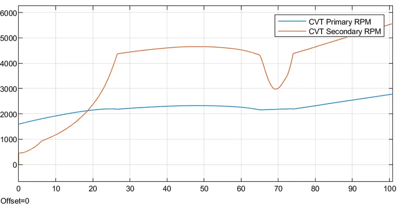

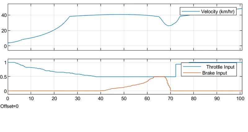
And the plot given below shows the comparison between the linear velocity of the vehicle and the throttle and brake force input over time

Conclusion:

Hence it can be concluded that

• In the model, the linear velocity of the vehicle is directly proportional to the throttle input and inversely proportional to the brake force input.
• The CVT ratio is directly proportional to the torque of the rear wheels and the speed of the vehicle.
• This model is primarily based on the study of the effect of the changes in the CVT ratio of the vehicle to the performance of the vehicle.