Project
AIM: - Carry out a system-level simulation of a BAJA All-Terrain Vehicle (ATV) Model.
The model created represents an All-Terrain Vehicle. This vehicle has low-pressure tires, the seat is straddled by the operator. The steering is controlled through a handlebar. The models are connected with a type of transmission system known as Continuously Varying Transmission (CVT).
CVT is an automatic transmission system that is capable of generating more power and providing a better fuel economy and a smooth ride as compared to the traditional automatic transmission system.
It allows the engine to run at a fixed rpm value while the vehicle is having different or varying speeds.
Some common Blocks used in the models are as follows:
Generic Engine Block: This block represents a general Internal Combustion Engine. The Engine can be spark-ignited or diesel. This block has 2 input ports and 3 output ports. The input port T is for the throttle level signal, 'B' is the mechanical rotational conserving port associated engine block.
The port F is the mechanical rotational conserving port associated with the engine crankshaft, P is the port of the physical signal of the engine power in Watts and FC port is the physical signal port for the fuel consumption in Kg/sec.
Variable Ratio Transmission Block: This block represents a physical gearbox that transfers the torque from the base shaft to the follower shaft or axle. This block is part of the subsystem named CVT.
Simple Gear Block: It is a Simscape model representing a gearbox that connects the base (driver shaft) to the follower (driven shaft) through a fixed gear ratio given by the user.
Vehicle Body Block: This block is a sub-system block in the given model. It represents the body of the vehicle along with all the different forces acting on the body. There are multiple input and output ports in this block.
The input ports take in the values of data like road inclination angle (‘beta’), Center of gravity of vehicle (CG), Mass (M), external Moment of Inertia (J), and Headwind speed (W).
The output ports are Longitudinal Velocity (V), Front axle normal Force (NF), Rear axle normal Force (NR)
H is the mechanical translational conserving port associated with the horizontal motion of the vehicle body.
Tire: this block is also a part of the sub-system named vehicle body. It represents a tire. There are four such block\s used representing the 4 tires of the vehicle.
Double Shoe Brake Block: this block represents a frictional shoe brake that presses against the rotating drum whenever actuated. F is the Actuating force signal port; S is the Drum shaft rotation and H is the Heat flow signal.
There are 6 different models in the given problem, namely:
- CVT Model.
- CVT Dashboard Model.
- CVT Data Model.
- CVT Mapped Model.
- CVT Model CVT Ratio_RPM.
- CVT Mapped Dashboard Model.
All the models are seen for the type of input signals, variations provided in each of the model and how these variations affect the output from the models.
MODEL 1: CVT Model
Main Model:
The block diagram of the main model is shown below:
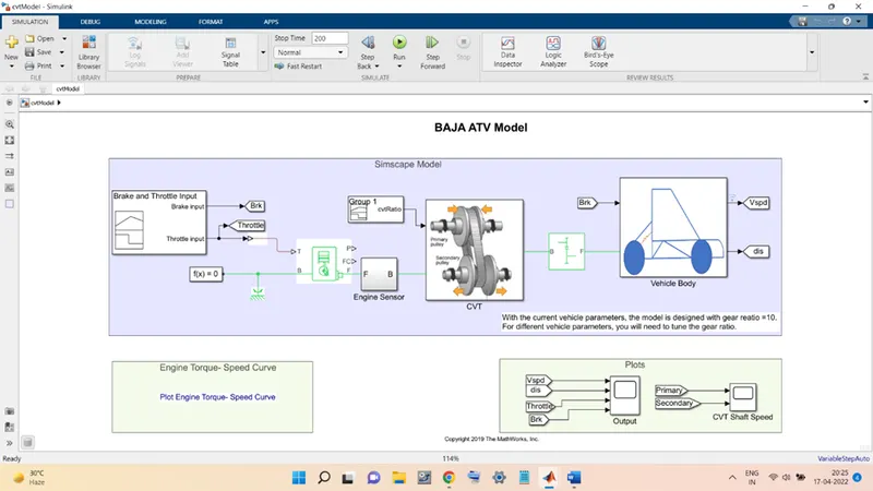
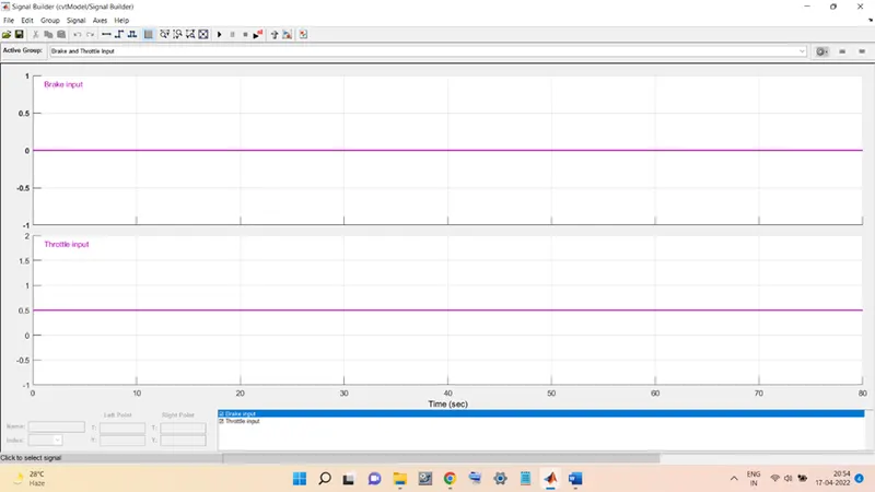
The input signals to this model are the Brake input and Throttle input supplied from the signal builder block. Both the inputs are constant throughout the simulation such that Throttle input = 0.5 and Brake input = 0.
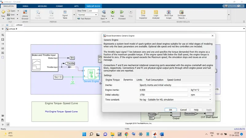
Next is the engine block, this block takes in the speed vector and torque vector as inputs. These are given by using MATLAB workspace.
The initial velocity value is kept at 1750 rpm, the engine inertia is taken to be 0.008 Kg-m^2, as shown in figure below:
This block will give the crankshaft rotational speed as an output signal. This signal is fed to the ideal rotational motion sensor block present in the ‘Engine Sensor’ block. This is a sub-system block as shown below:
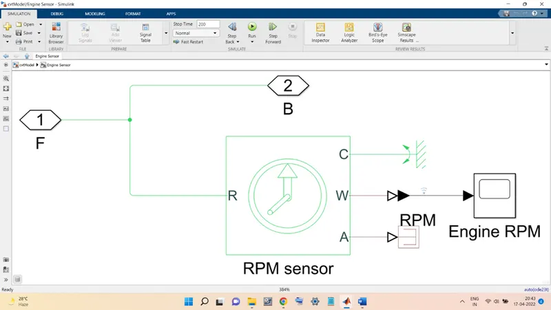
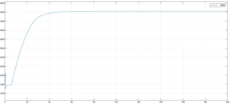
This sensor output is fed to a scope, the scope will plot the rpm feed against time. The plot so obtained is shown below:
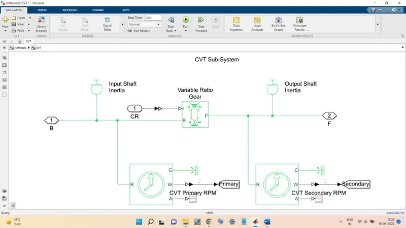
The second branch of the input rpm feed numbered ‘1’ is sent to the next sub-system block named, ‘CVT’. The block diagram is shown below:
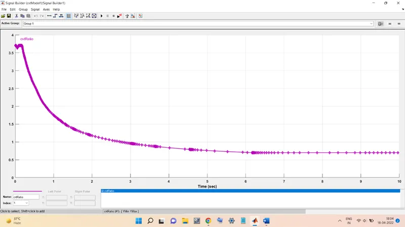
Since the CVT ratio (the second input to the CVT sub-system) is time-dependent so, the CVT ratio is generated using a signal builder block as shown below:
After adding the inertia effects of the input shaft, the rpm signal is fed to the Variable Gear Ratio block by the name ‘B’. the second input, CVT Ratio, is fed to it by name ‘CR’.
An Ideal Rotational Motion Sensor is connected to the rpm input line and the output of this sensor is sent to, using the GO TO Block, scope named as ‘CVT Shaft Speed’.
The output from the Variable Ratio Gear block is the rpm generated at the Follower Shaft.
An Ideal Rotational Motion Sensor is connected to the output rpm line, it measures the rpm value and sends the output values to a scope named ‘CVT Shaft Speed’ using a GO TO block.
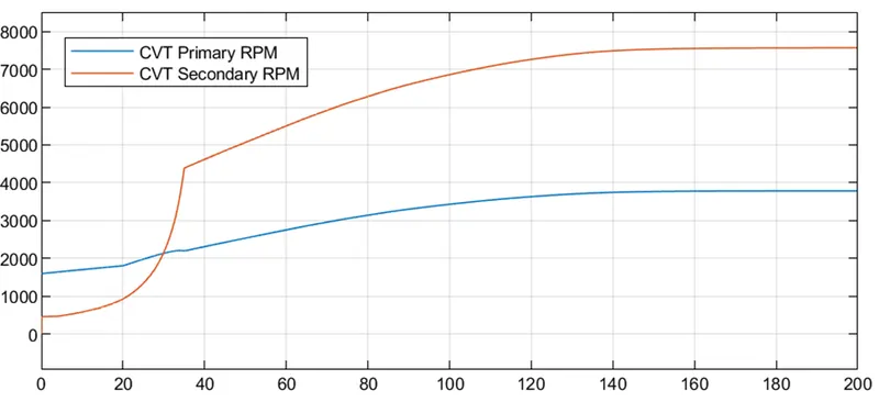
The scope CVT Shaft Speed will plot the primary and secondary speed of the CVT against time for better understanding.
The output rpm signal of the follower shaft id then fed to the block named, Simple Gear. This block is a simple gear with fixed gear ratio and corresponding to the gear ratio value supplied by the user the rpm feed will get modified respectively.
The output rpm feed from Simple Gear block is the sent to the next sub-system block named as, Vehicle Body. The block diagram is shown below:
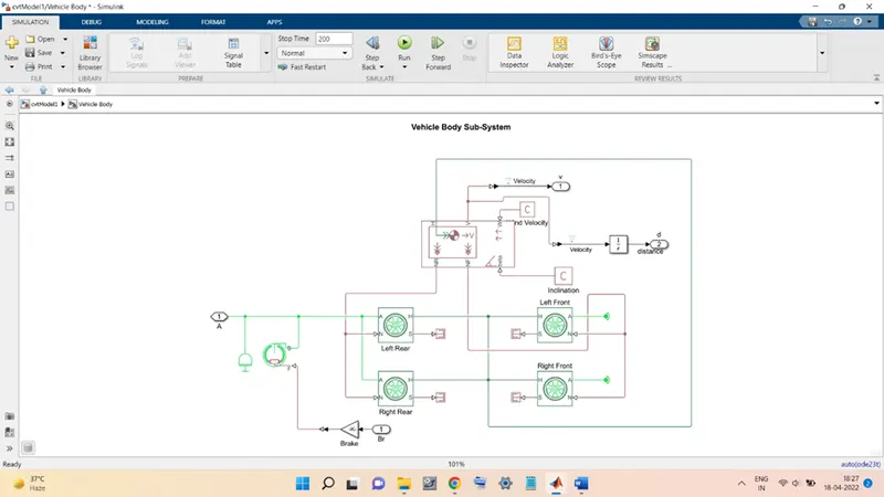
The rpm feed from the Simple Gear block goes to the Vehicle Body block. In this block, the rpm is supplied as input to the four tires as shown in the figure. Before that:
The brake input signal, using the ‘From’ block, is supplied to the gain block (named ‘Brake’) where it is multiplied by a scalar of magnitude 1000. The output from the gain block is first converted into the physical signal using the ‘Simulink-PS Converter’ block and then fed to the ‘Double-Shoe Brake’. The input to this block is the force supplied through the port ‘F’ and the output is the frictional torque acting upon the drum shaft. This output is obtained from the port ‘S’.
The parameters involved in the brake shoe block like, drum radius, actuator location radius, viscous friction coefficient, contact friction coefficient, etc. are all supplied by the user into the block.
The Inertia block is also attached to the input rpm line to include the inertia effects consideration.
The Tire blocks are characterized for longitudinal behavior by using the ‘Tire Magic Formula’. The block diagram of the Tire is shown below:
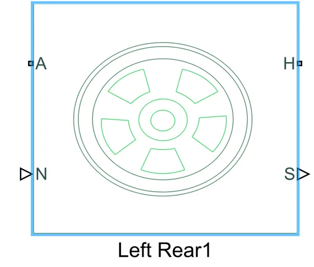
‘A’ port receives the input rpm signal, ‘H’ is a mechanical translational conserving port for the wheel hub through which the thrust developed by the tire is applied to the vehicle. ‘N’ is the input port that applies the normal force acting on the tire. ‘S’ port gives value for the slip present at the tire.
All the output signals (H) from the tires block are then sent to the Vehicle Body block (the red box just above the tire blocks). This block represents the body of the ATV. All the input parameter values are supplied to the block depending upon the user. The output from this block is the vehicle velocity, obtained at the port named, ‘V’.
This output is then split into two branches, the first branch signal is first converted to Simulink signal from the physical signal, and then with the help of 'GO TO' block is supplied to the scope named, ‘Output’.
The second branch, after being converted to Simulink signal, first is integrated and the output of integration is now the distance traveled by the vehicle. This signal is again supplied to the scope Output, to see the variation with respect to the time.
This completes the flow process of the signal from start to end and this is the basic flow process seen for all different models given in the problem. The only thing that changes is the type of input given and the respective output obtained from those inputs for different models. As discussed below:
OUTPUTS:
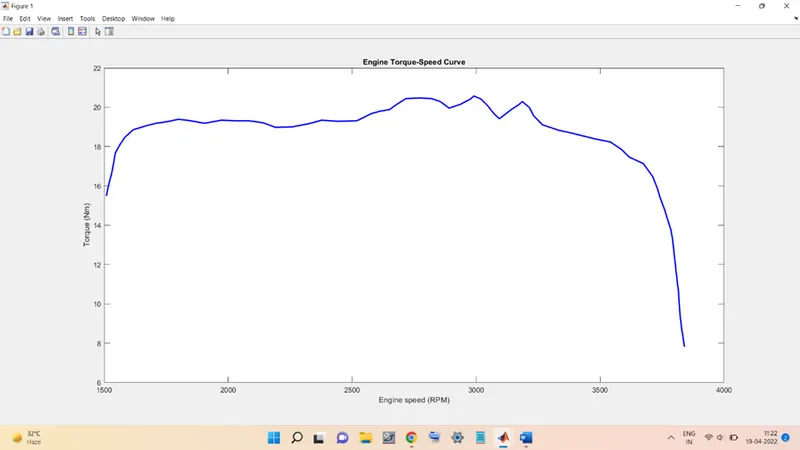
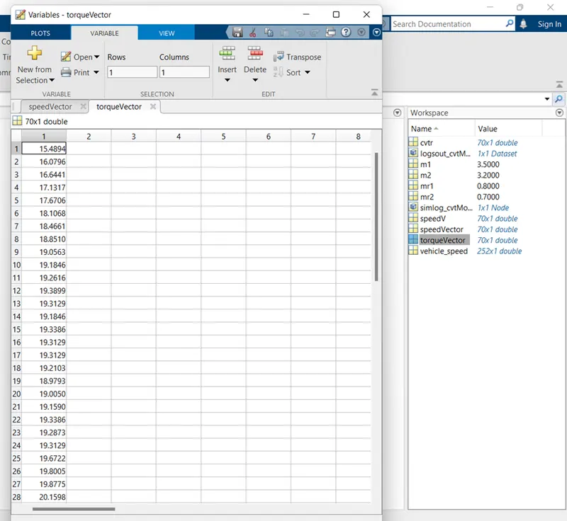
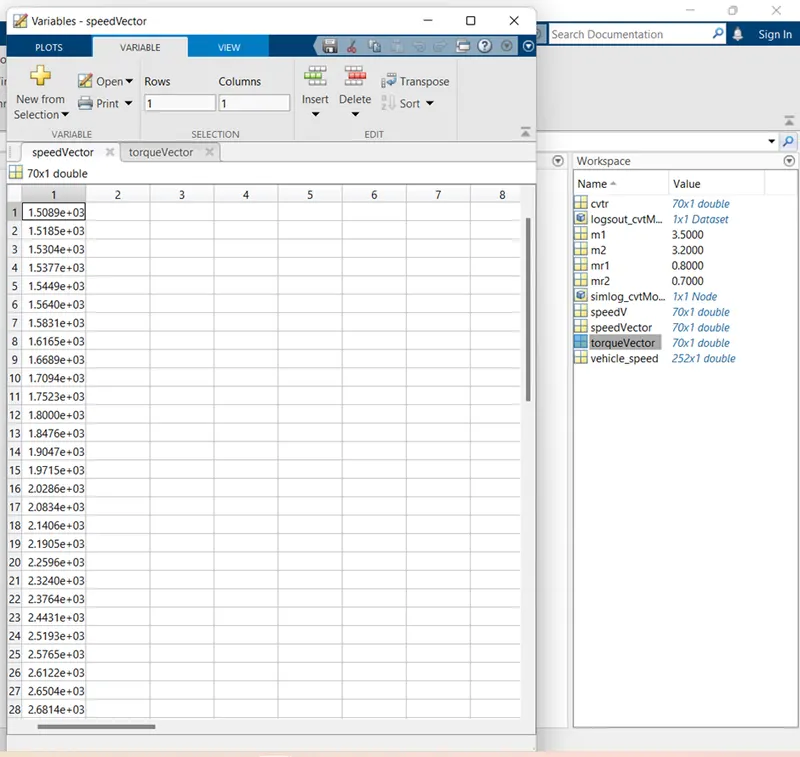
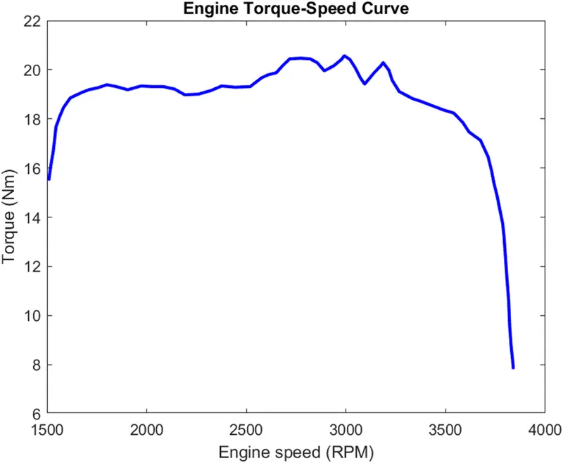
Engine Torque vs RPM curve: This is the plot between the Torque Vector and the Speed Vector, supplied as inputs to the Generic Engine The values of both the vectors are obtained from MATLAB workspace as shown below:
Vehicle Velocity, Distance, Throttle, and Brake vs Time: This is the plot obtained from the scope named as, Output. The plot is given below:
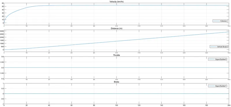
From the above plot, the velocity is seen to increase for the initial time and then the curve flattens and is constant for the rest of the time. This is due to the fact that the throttle is kept constant equal to 0.5 and the gear ratio also gets constant after some time.
CVT Primary and Secondary RPM vs Time: This plot is obtained from the scope named CVT Shaft Speed. The plot is shown below:
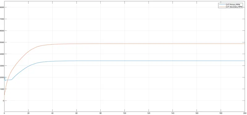
During the early phase of the simulation, from the CVT ratio plot, it is seen that the CVT ratio decreases from a higher value to a lower value, and the gear ratio is greater than 1 as a result, the secondary rpm is less than the primary rpm. But after 6 secs, the CVT ratio value is seen to get constant and less than 1 (around 0.7) as a result the secondary rpm is now greater than the primary rpm.
MODEL 2: CVT Model with DASHBOARD
The basic structure of this model is the same as that of the previously discussed model, the signal flow in this model is also the same as that in the previous model. The only difference in this model is that the input signals, throttle, and Brake input can be tuned using the Dashboard. As shown below:
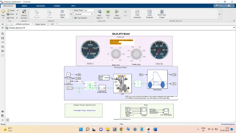
The Dashboard contains 2 Dials (at the left and right corners) and 2 Knobs (in middle). The Dial in the left corner will indicate the RPM value and the dial on the right will show the Velocity value.
The knobs are used to change the values of the input signals. The Brake Input knob is used to change the Brake input signal value and the Throttle Input knob will change the Throttle input signal value.
The simulation time is kept at infinity in this model and in this simulation, first, the Throttle Input will be changed from the value 0.5 to 0.8 and then again back to 0.5 keeping the Brake Input value constant (zero) and later the Throttle Input will be constant at b and the Brake Input will be changed from 0 to 0.2 and then back to 0.
The outputs obtained for this model are shown below:
OUTPUTS
Engine Torque vs RPM curve: The values of both parameters are obtained in the same fashion as obtained in the previous model. The plot is also the same plot as shown below:
Vehicle Velocity, Distance, Throttle, and Brake vs Time: The plot is obtained by varying the Throttle and Brake input values while the simulation is running. The plot is shown below:
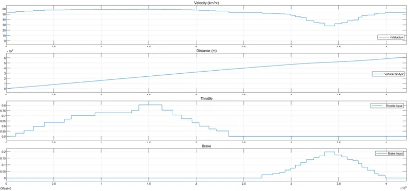
As can be seen from the plot as the Throttle input increase the speed also increase and speed decreases with the decrease in the Throttle input. Also, when the Brake input is increased the speed reduces, and with the decrease in the Brake Input the speed again gets increased.
CVT primary and Secondary RPM vs Time: The plot shows the variation of Primary and Secondary RPM with Time as the 2 input signals are tuned while the simulation is still running. The plot is shown below:
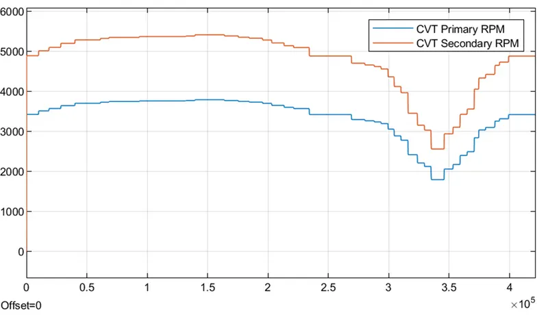
In the plot also, with the increase in Throttle Input the RPM in primary and secondary shafts increases, and both decrease with its decrease. Similarly, with an increase in Brake Input, the RPM values of both the shafts reduce, and with a decrease in Brake Input the RPM values are seen to increase.
MODEL 3: CVT Model with Data
The block diagram of this model is shown below:
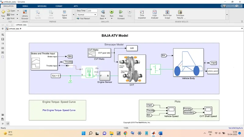
The basic structure of this model is also similar to the first model itself. The signal flow process is also the same as that explained in the first model.
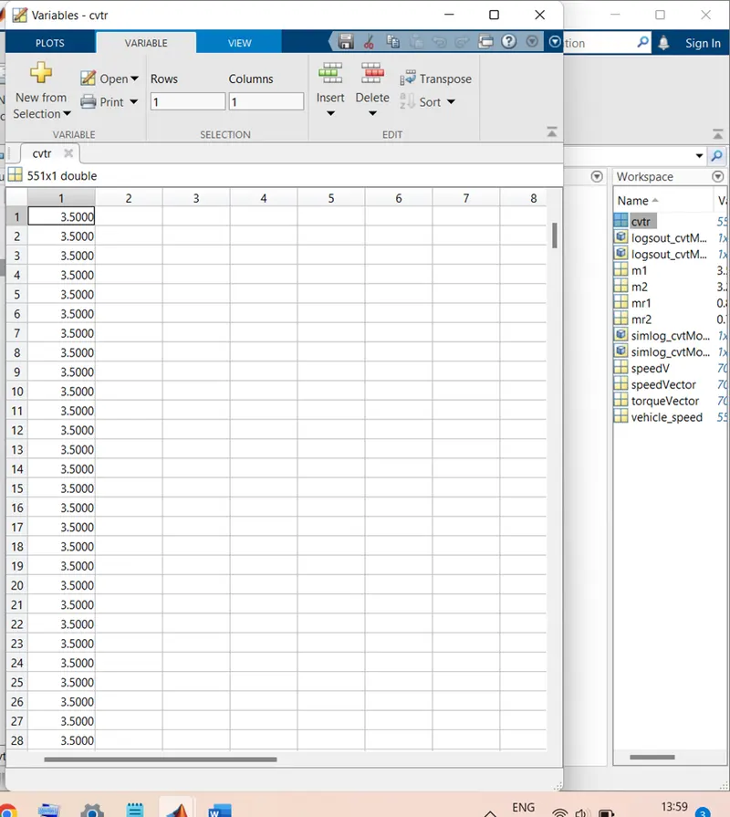
The only difference in this model is that there are two branches of the output signal of the block named, ‘CVT Ratio’. One branch is supplied to the CVT block as done in the first model also. The second branch is supplied to the ‘To Workspace’ block. This block is designed to construct an array or time-series or structure in the MATLAB workspace of the data received as input. Thus, in this model, this block will create an array from the data supplied from the CVT Ratio block and the name of this array is ‘cvtr’.
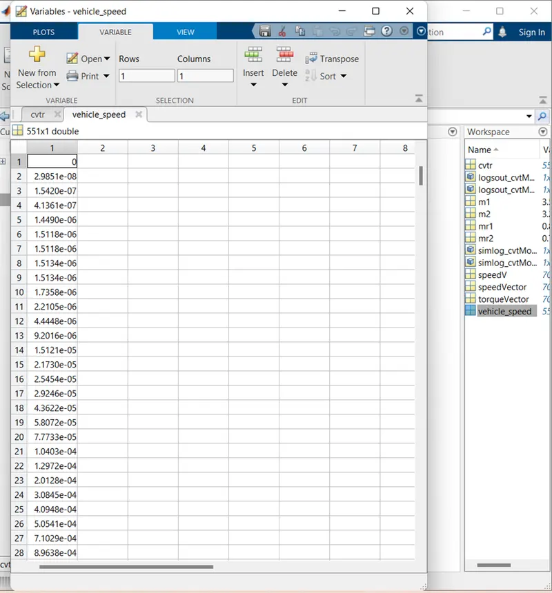
The same thing is also done for the output from the ‘Vehicle Body’ sub-system. One branch named, ‘Vspd’ is given as input to the scope ‘Vehicle Speed’. The other branch is sent to the block ‘To Workspace’ in which the data will be converted into an array called ‘vehiclespeed’.
OUTPUTS:
Engine Torque vs RPM curve:
Vehicle Velocity, Throttle, and Brake vs Time:
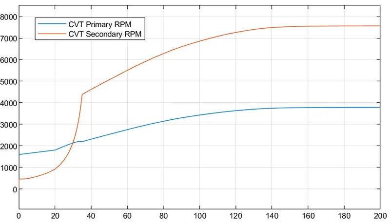
CVT primary and Secondary RPM vs Time:
The CVT Ratio array ‘cvtr’:
The vehicle speed array, ‘vehicle_speed’:
MODEL 4: CVT Model MAPPED
The block diagram for this model is shown in the below figure:
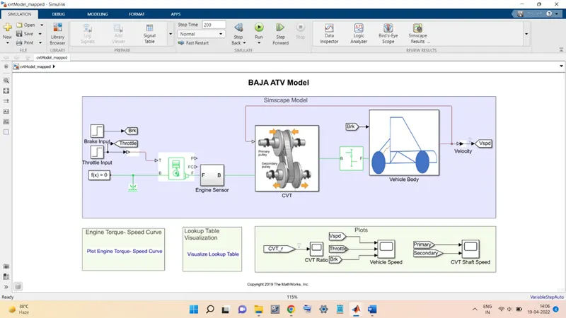
The basic model structure remains the same and the signal flow process is also the same. The changes done in this model are:
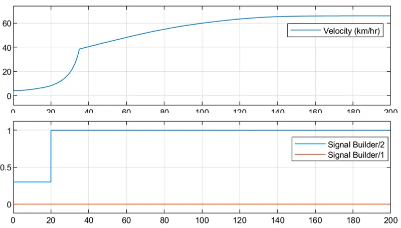
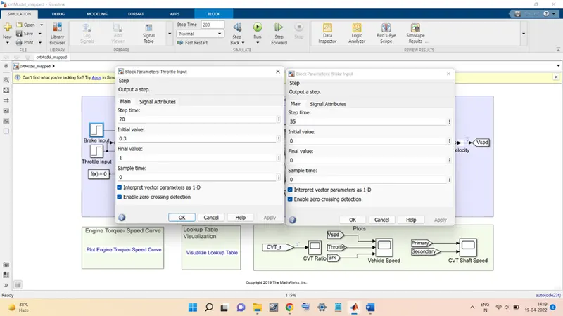
The throttle Input signal, in this model, is generated with the help of a ‘step’ block. The throttle input value is 3 for the first 20 seconds and then changes to 1 at a time equal to 20 seconds and remains there for the rest of the simulation. The same is done for the Brake Input signal but its value is kept at zero throughout the simulation.
CVT gear ratio, in this model, is generated with the help of a block ‘Look-Up Table’. A look-up table is an array of data that maps the input values to the output values, thereby approximating a mathematical function. The modified CVT sub-system is shown below:
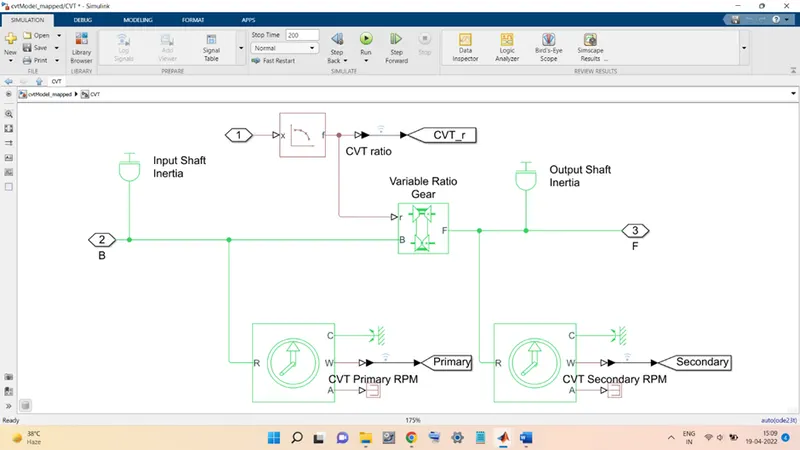
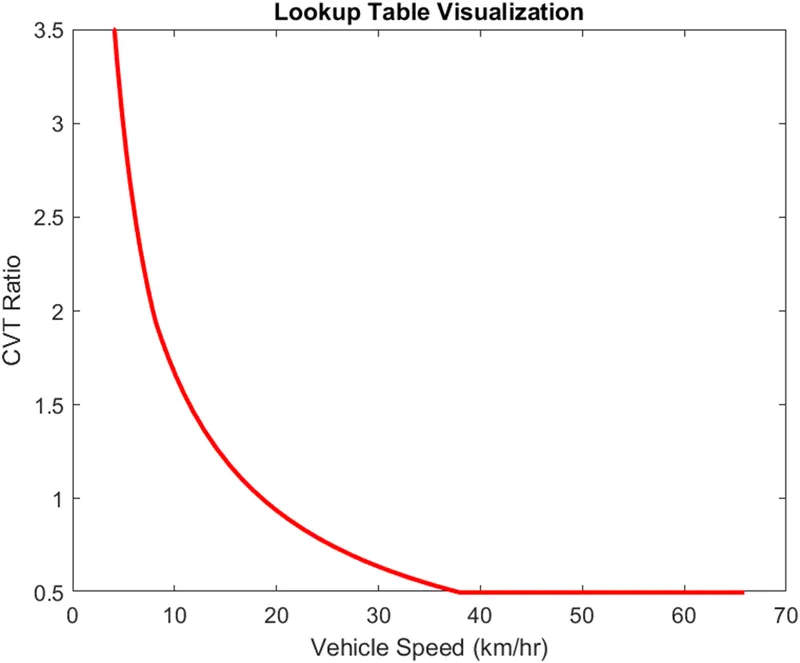
The output of the ‘Vehicle Body’ sub-system is the velocity of the vehicle, this velocity is taken as the input to the Look-up Table block and the look-up table block will give the ‘CVT Gear Ratio’ as the output for the corresponding vehicle velocity values. The output from the look-up table block is split into two branches such that, one branch is fed to the ‘Variable Ratio Gear’ block and the other branch is supplied to a scope ‘CVT Ratio’ with the help of the ‘GO TO’ block.
The plot obtained with the help of the ‘Look-up Table’ block is shown in the figure below:
OUTPUTS:
Engine Torque vs RPM curve:
Vehicle Velocity, Throttle, and Brake vs Time:
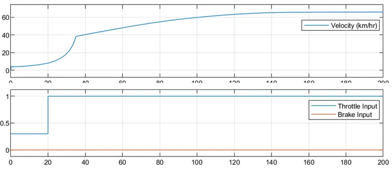
From the above figure, it can be seen that the rate of increase of the vehicle velocity during the early phase (approx. till 36 seconds) is more than that observed during the later phase where the rate of increase is smoother than early phase rate.
CVT Gear Ratio:
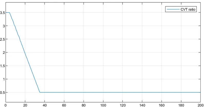
The CVT Ratio obtained from the look-up table when plotted against the time is shown in the figure below:
CVT primary and Secondary RPM vs Time:
MODEL 5: CVT Model CVT Ratio_RPM
This model is also same as the first model and the signal flow mechanism is also the same. The only change in this model as compared to the first model is that the CVT Gear Ratio values are obtained using a block ‘Look-Up Table’.
This method was also used in the model number 4, however, in the model 4, the input to the ‘Look-up Table’ block was the Vehicle Speed, but in this model the input to the ‘Look-up Table’ block is the ‘Engine RPM’ value which is the output signal from the ‘Engine Sensor’ sub-system.
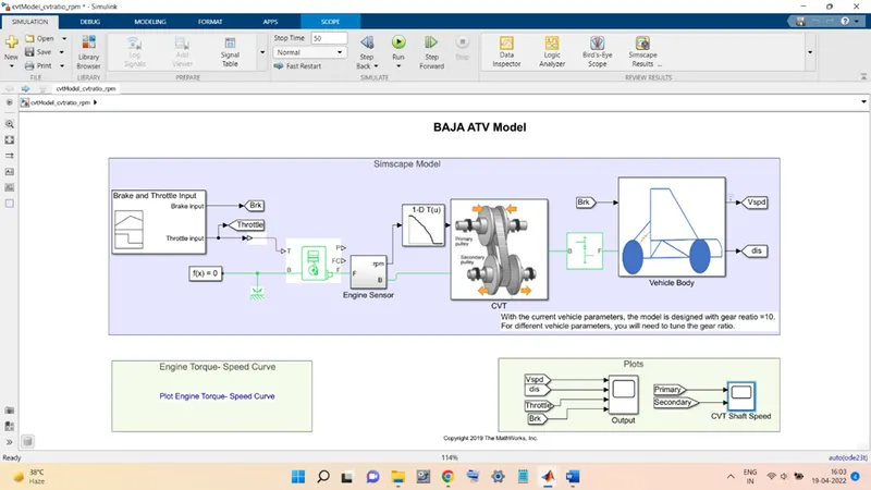
The model block diagram is shown below:
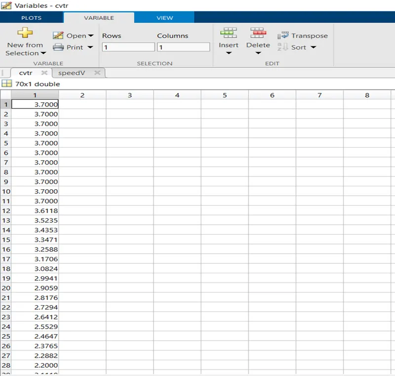
The CVT Ratio array obtained from the look-up table can be seen in the figure below:
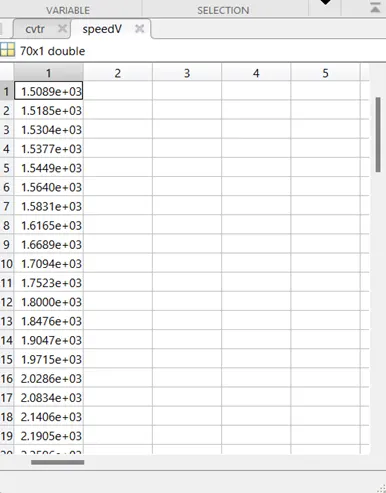
The ‘speedV’ values stored in the MATLAB workspace are also shown in the figure below:
OUTPUTS:
Engine Torque vs RPM curve:
Vehicle Velocity, Distance, Throttle, and Brake vs Time:
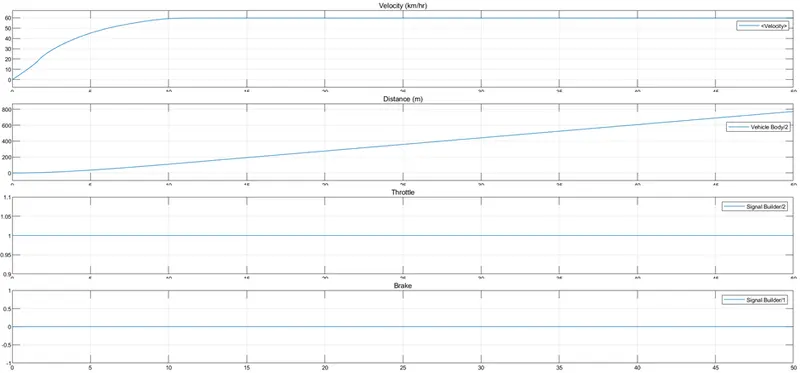
In this model, the Throttle Input value is kept at 1 for the entire simulation and the value of Brake input is kept at zero.
The Vehicle Velocity increases from zero to 60 for the first 10 seconds of the time interval and then its value is constant for the rest simulation period.
CVT primary and Secondary RPM vs Time:
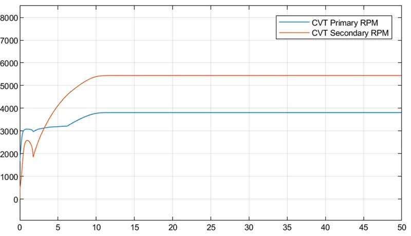
The RPM in both primary and secondary shafts gets constant for time after first 10 seconds of the simulation.
MODEL 6: CVT Model Dashboard MAPPED
The model, in this case, is basically the same as the first model of the vehicle, the signal flow arrangement is also the same as that in the first model.
The difference in this model is that:
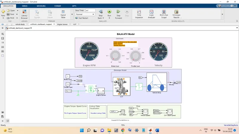
First, the input signals Throttle and Brake Inputs can be tuned while the simulation is running with the help of the modulating knobs shown in the above figure. The ‘Brake Input’ knob is used to change the value of the Brake Input signal, and the ‘Throttle Input’ knob changes the value of the Throttle Input signal. This is the same as done in MODEL 2.
Second, the CVT Gear Ratio values are obtained using the ‘Look-Up Table’ block. The input signal to the ‘Look-up Table’ block is ‘Vehicle Speed’, output from the Vehicle Body sub-system. This is the same as done in MODEL 4.
This model can be said as the combination of Model 2 and Model 4.
To see the variation of output, the Throttle Input signal is varied from the initial value of 0.3 to 0.8 and then back to 0.3, meanwhile the Brake Input is kept constant at zero.
Then the Throttle Input is kept constant and the Brake Input signal is varied from 0 to 0.3 and then back to zero.
The outputs obtained for this model are as follows:
OUTPUTS:
Engine Torque vs RPM curve:
Look-Up Table of CVT Ratio:
Engine RPM vs Time:
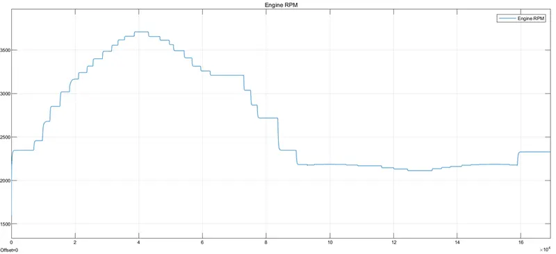
In the figure, the left side peak is depicting the variation of the Engine RPM with respect to the Throttle Input value. It is seen that as the Throttle Input value is increased the RPM of the Engine also increases and as the throttle value reduces the RPM also decreases.
The right portion of the figure shows the Engine RPM variation with respect to the Brake Input signal. The Engine RPM is seen to be very less affected by variation in the Brake Input values.
CVT Ratio vs Time:
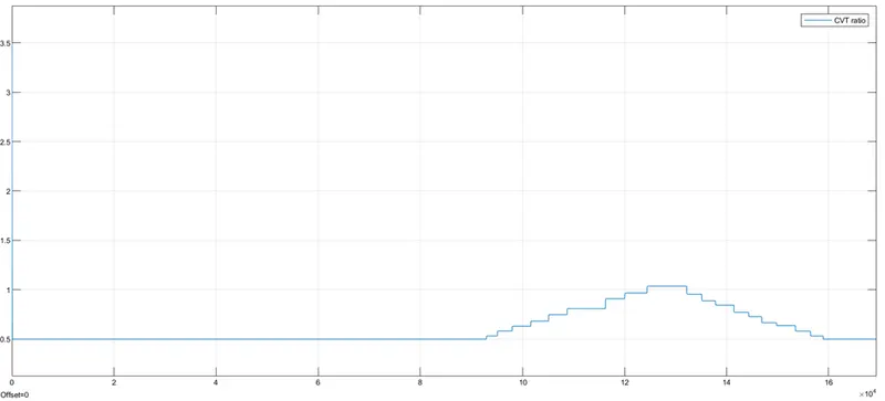
From the above figure, it is seen that the CVT Ratio shows no variation with respect to the change in the Throttle Input signals.
The CVT Ratio is seen to increase with the increase in the Brake Input values and decrease also as its value reduces.
Vehicle Velocity, Throttle, and Brake Input vs Time:
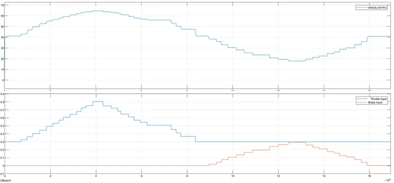
The Vehicle Velocity is seen to increase with the increase in the throttle input value and it decreases with a decrease in the throttle input value.
Also, velocity shows the inverse relation with the brake input signal as seen from the above figure.
CVT primary and Secondary RPM vs Time:
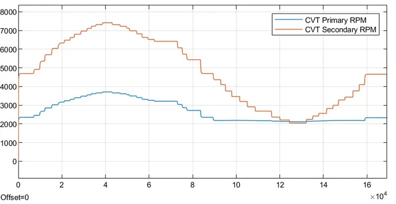
Both the Primary and the Secondary shaft RPM are seen to show a direct relationship with the Throttle Input signal as can be seen from the figure.
The secondary RPM is seen to have an inverse relation with the Brake Input signal.
However, the primary RPM is very minutely affected by the Brake Input signal, since the curve is almost horizontal as seen in the figure.