Simulation of an all-terrain vehicle using BAJA ATV Model

TYPES OF MODEL STUDIES :

1. BAJA ATV model without Dashboard (cvt Model)
2. BAJA ATV model - Data Extraction (cvt Model)
3. BAJA ATV model with Dashboard (cvt Model)
4. BAJA ATV model - Mapped Lookup Table without Dashboard (cvt Model_mapped)
5. BAJA ATV model - Mapped Lookup Table With Dashboard (cvt Model_Dashboard_mapped)

Introduction :

ALL TERRAIN VEHICLE :

An All Terrain Vehicle (ATV) is defines as a motorized off - highway vehicle defined to travel on four low - pressure or non - pneumatic tires, having a seat designed to be straddled by operator and handlebars for steering control.

CVT :

A CVT or Continuously Variable Transmission (CVT) is an automatic, Single-speed and gearless Transmission that can shift through an infinite number of gear ratios. This contrasts with other transmissions that provide a limited number of gear ratios in fixed steps. The Flexibility of a CVT with suitable control may allow the engine to operate at a constant RPM while the vehicle moves at varying Speeds.

1. BAJA ATV model without Dashboard (cvt Model) :

Main Model :

A Simulink model for BAJA ATV Model is shown.

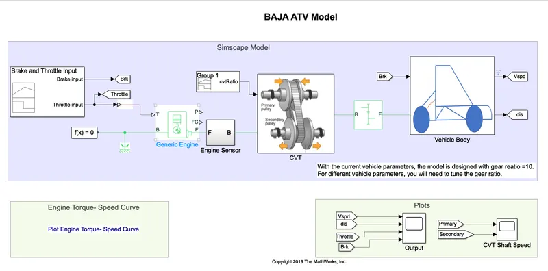
The model consist of common blocks as follows :

Signal Builder :

• The Signal Builder block allows you to create interchangeable groups of piecewise linear signal sources and use them in a model.
• You can Quickly Switch signal groups into and out of a model to facilitate testing.

Generic Engine :

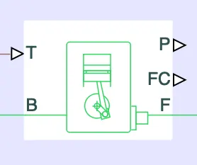
• Represents a system-level model of spark-ignition and diesel engines suitable for use at initial stages of modeling.
• A thottle physical signal input specifies the normalized engine torque.
• Optional dynamic parameters include crankshaft inertia and response time lag.
• Connections F and B are mechanical rotational conserving ports associated with the engine crankshaft and engine block, respectively.
• Connections P and FC are physical Signal output ports through which engine power and fuel consumption rate are reported.
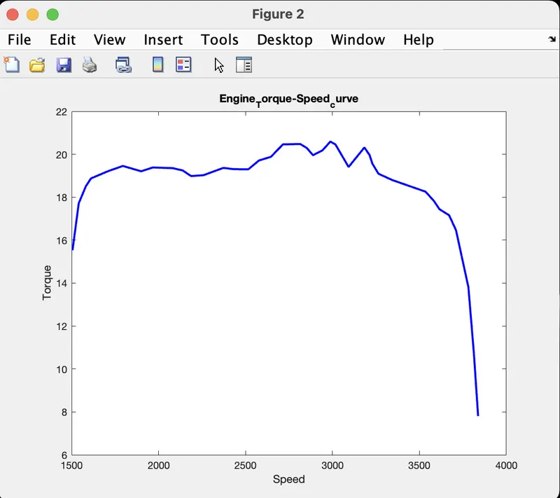
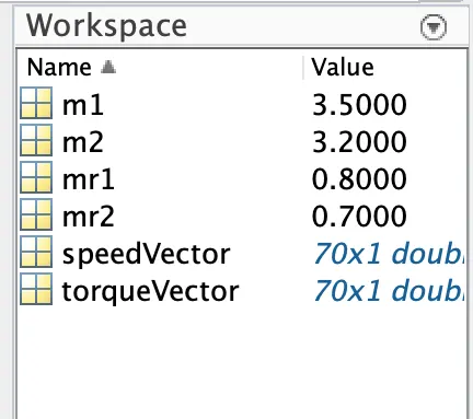
• Speed vector and Torque vector are the assigned parameters.

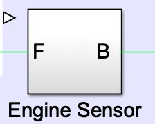
Engine Sensor :

Ideal Rotational Motion Sensor :

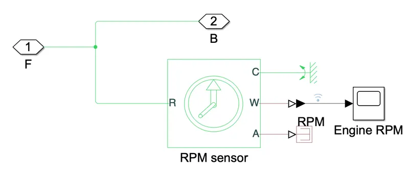
• The block represents an ideal mechanical rotational motion sensor, that is, a device that converts an across variable measured between two mechanical rotational nodes into a control signal proportional to angular velocity or angle.
• The sensor is ideal since it does not account for inertia, friction, delays, energy consumption, and so on.
• Connections R and C are mechanical rotational conserving ports and connections W and A are physical Signal output ports for velocity and angular displacement, respectively.

Simple Gear :

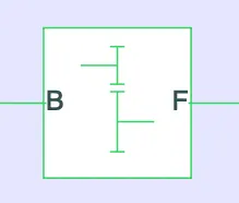
The Simple Gear Block represents a gearbox that constrains the connected driveline axes of the base gear, B, and the follower gear, F, to corotate with a fixed ratio that is specified.

The Follower-base gear ratio is

`gFB=(rf)/(rB)=(NF)/(NB)`

Where,

• `N_B` is number of teeth in the base gear
• `N_(F)` is number of teeth in follower gear

Variable Ratio Transmission Block :

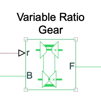
• Represents a variable ratio gearbox such as implemented by mechanical belt CVT, electric, or hydraulic transmissions.
• The Physical signal input 'r' defines the ratio of input to output angular shaft velocities.
• Connections B (base) and F (follower) are mechanical rotational conserving ports.
• Specify the relation between base and follower rotation directions with the output shaft rotates parameter.

Inertia :

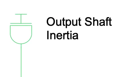
• This Block represents an ideal mechanical rotational inertia.
• The block has one mechanical rotational conservation port. The Block positive direction is from its port to the reference point.
• This means that the inertia torque is positive if the inertia is accelerated in a positive direction.

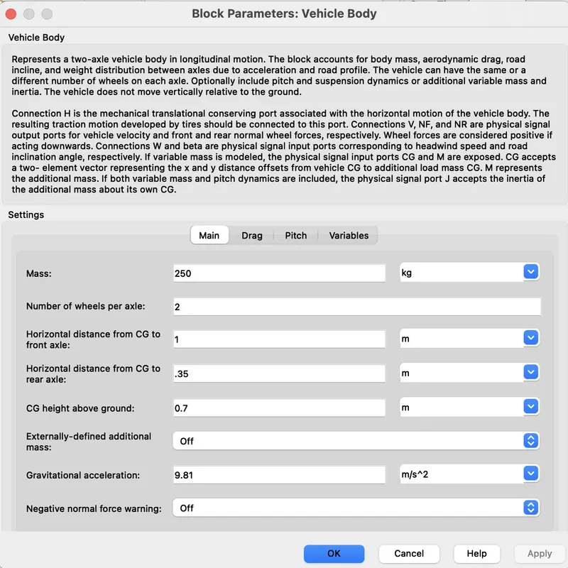
Vehicle Body :

• The Vehicle Body block represents a two-axle vehicle body in longitudinal motion. The vehicle can have the same or a different number of wheels on each axle.
• Example : Two wheels on front axle and one wheel on the rear axle. The Vehicle wheels are assumed identical in size. The vehicle can also have a center of gravity (CG) that is at or below the plane of travel.
• The block accounts for boby mass, aerodynamic drag, road incline, and weight distribution between axles due to acceleration and road profile. Optionally include pitch and suspention dynamics. The Vehicle does not move vertically relative to ground.
• The block has an option to include an externally-defined mass and an externally-defined inertia, The mass, inertia, and center of gravity of the vehicle body can vary over the course of simulation in response to system changes.

Double Shoe Brake :

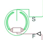
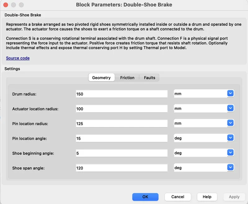
• The Double-Shoe Brake block represents a frictional brake with two pivoted rigid shoes that press against a rotating drum to produce a bracking action. The rigid shoes sit inside or outside the drum in a diametrically opposed configuration.
• A positive actuating force causes the girid shoe to press against the rotating drum. Viscous and contact friction between the drum and the rigid shoe surface cause the rotating drum to decelerate.
• Double-Shoe brakes provide high bracking torque with small actuator deflections in applications that include motor vehicles and some heavy machinery.
• The model employs a simple parameterization with readily accessible brake geometry and friction parameters.

Tire :

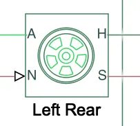
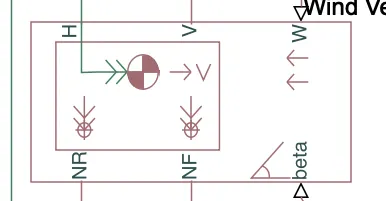
• Represents the longitudinal behavior of a highway tire characterized by the tire magic formula. The block is built from Tire-Road Interaction (Magic Formula) and Simscape Foundation Library Wheel And Axle blocks.
• Optionally, the effects of tire inertia, stiffness, and damping can be included. Connection A is the mechanical rotational conserving port for the wheel axle.
• Connection H is the mechanical translational conserving Port for the wheel hub through which the thrust developed by tire is applied to the vehicle.
• Connection N is a physical signal input port that applies the normal force acting on the tire. The Force is considered positive if it acts downwards. Connection S is a physical signal output port that reports tire slip.
• Optionally expose physical signal port M by setting parameterize by to physical signal Magic Formula coefficients. Physical signal port M accepts a four-element vector corresponding to B, C, D,and E Magic Formula coefficients.

Torque vs Speed characteristics :

INPUTS :

Brake and Throttle input :

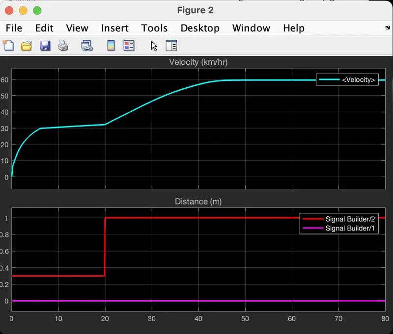
Brake : Input is constant i.e., Zero through out the time of 80 sec.

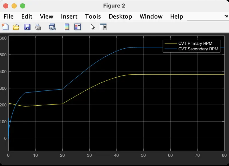
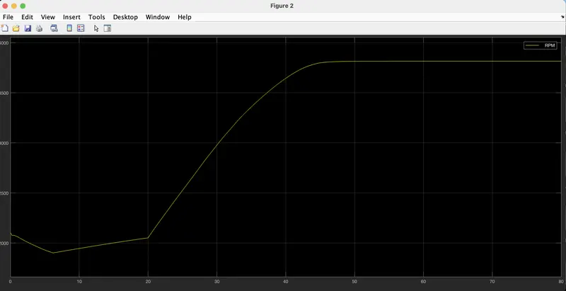
Throttle : Input is 0.3 for first 20 sec, acclerates to 1 at same and remains constant throughout the remaining time till 80 sec.

CVT Ratio :

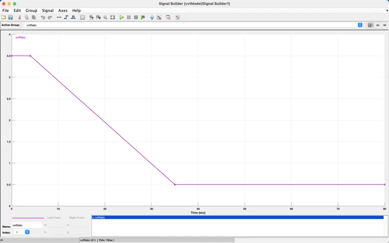
The CVT gear ratio 3.5 for the first 4 sec, then drops down to 0.5 till 35 sec and remains the same till 80 sec.

OUTPUT :

Velocity :

CVT Shaft Speed :

Engine Speed :

2. BAJA ATV model - Data Extraction (cvt Model_data):

Main Model :

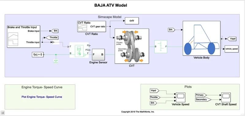
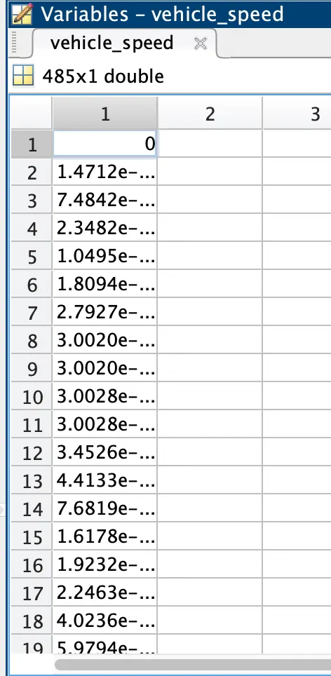
The Model Workflow process is same as the process of ' BAJA ATV model Without Dashboard '. The small addition is that the CVT Ratio and Vehicle Speed data are extracted using ' To Workspace ' block.

Before Workspace Block :

After Workspace Block :

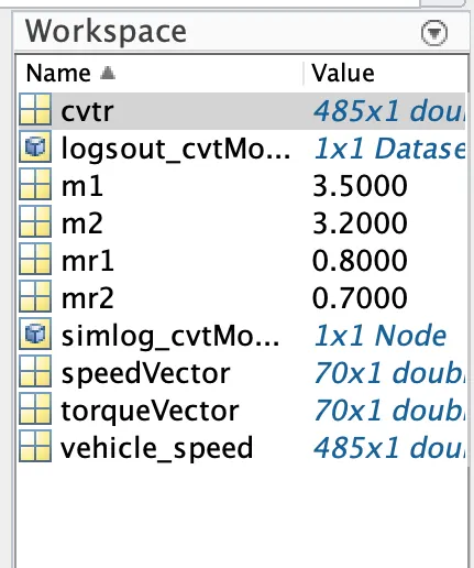
cvt_ratio Data :

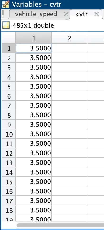
vehicle_speed Data :

3. BAJA ATV model with DashBoard (CVT Model_Dashbord) :

Main Model :

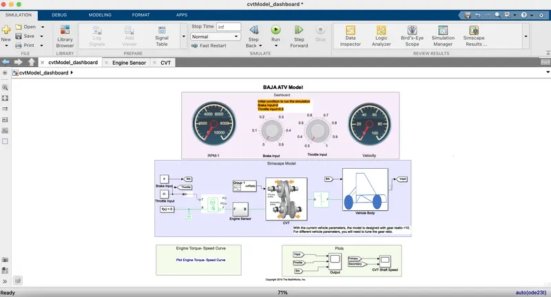
Explanation :

The model workflow process is the same as process of ' BAJA ATV model without Dashboard '. But the Throttle and Brake input are controlled by the user with knobes.

Engine Speed Plot :

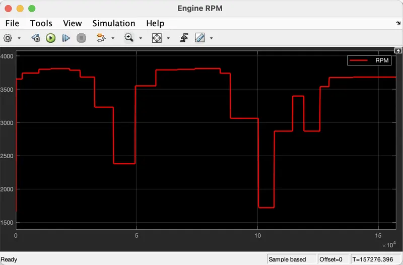
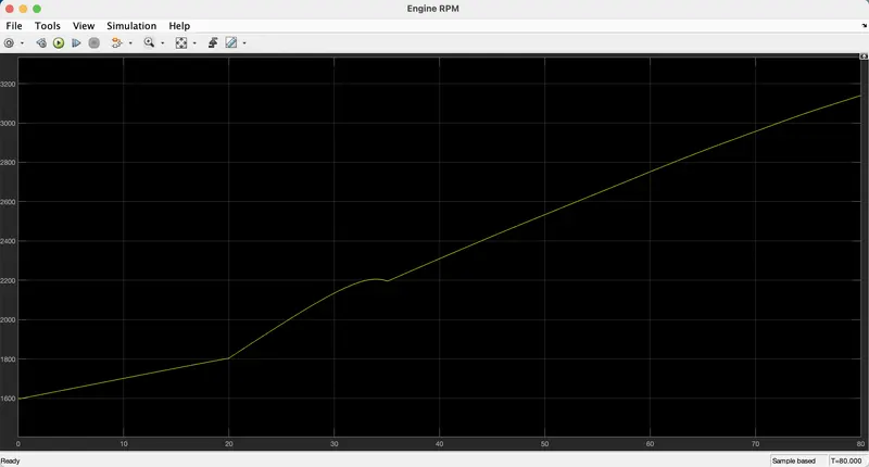
The Engine Speed is generated according to the inputs like throttle, brake, Torque and Speed Vectors.

The Run time is not given so that Throttle Input and brake Input are controlled by User.

The Step up is Throttle and Step down is brake Input.

CVT Speed Reduction Plot :

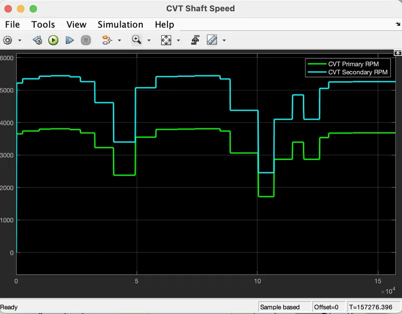
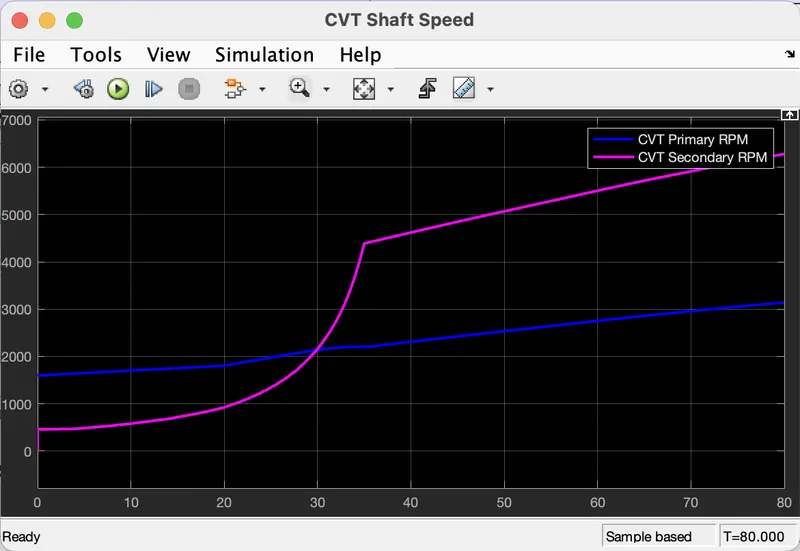
The CVT Speed Reduction Plot shows that at constant reduction ratio of 0.7 is applied to these larger time frame.

It can be werified by taking 5200 constant RPM and dividing it by 0.7 = 3800 RPM which verifies the plot.

Speed Vs. Throttle Input :

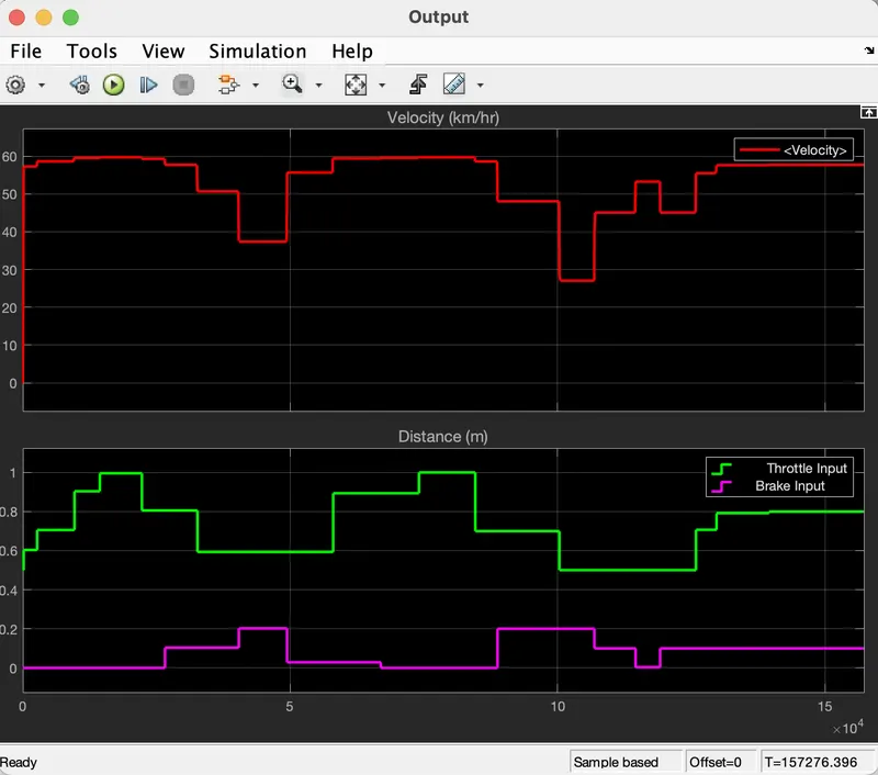
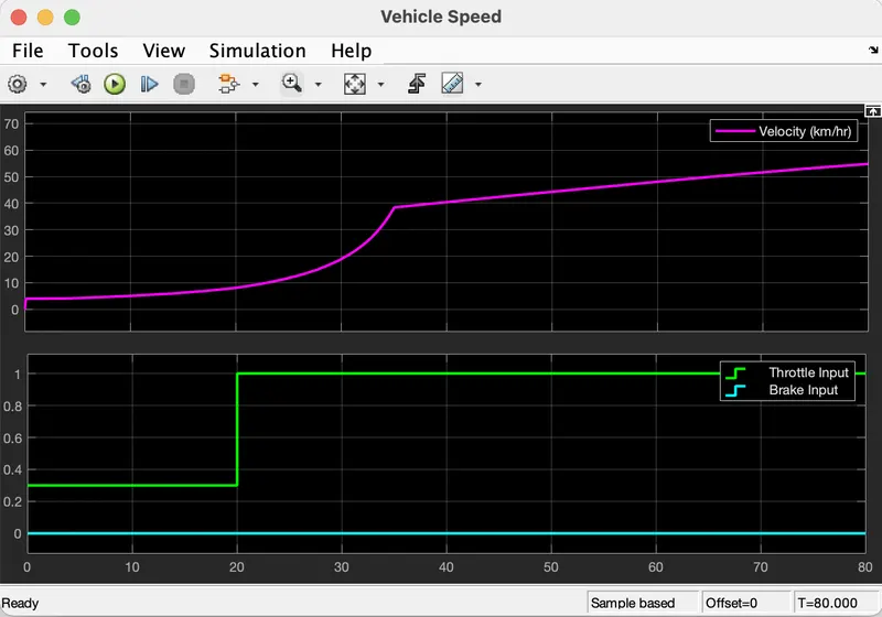
The Graphs Shows we can infer that the vehicle is accelerating while Throttle is applied (Step Up) and decelerated while brake is applied (Step Down).

The Constant speed areas represent no changes in throttle or brakeing.

4. BAJA ATV model - Mapped Lookup Table without Dashboard (cvt Model_mapped) :

Main Model :

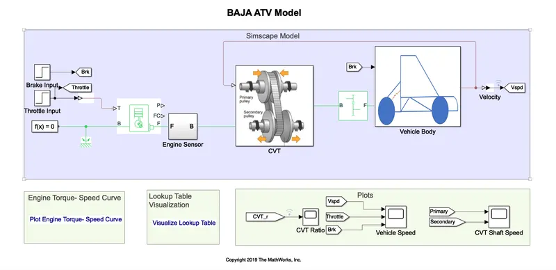
Explanation :

The Model workflow process is same as the process of ' BAJA ATV model without Dashboard ' except that it used insead of Step Input Blocks for Both brakeing And Throttle Input are used.

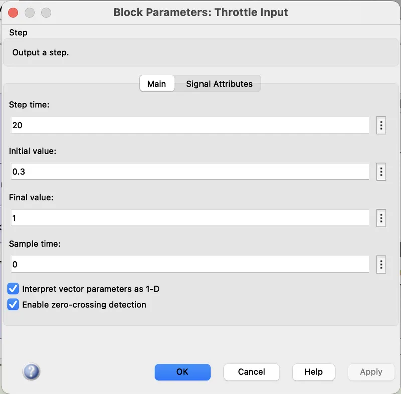
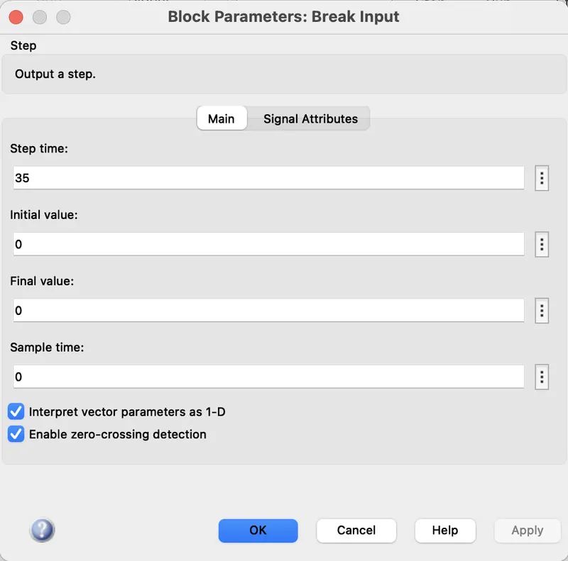
At 35 sec the brake input will take a step of value '0' and at 20 sec throttle input will increases from 0.3 to 1 then remains constant throughout.

CVT SUBBLOCK :

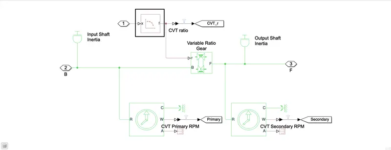
The CVT subblock is same as previous model " BAJA ATV model without Bashboard ". But instead of Signal Builder Block for CVT Ratio 2-D Lookup Table is used.

The interpolations and extrapolation methods are set to linear. It needs to be loaded in the workspace having the file name as Lookuptable_data.mat.

Lookup Table :

A lookup table is an array of data that maps input values to output values, thereby approximating a mathematical function.

Given a set of input values, a lookup operation retrieves the corresponding output values from table.

If the lookup table does not explicitly define the input values, Simulink can estimate an output value using interpolation, extrapolation, or rounding.

CVT ratio Plot :

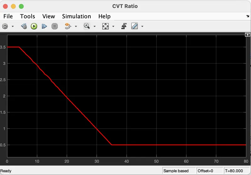
When we compare above plot, the ratio varies from 3.5 to 0.5 within time span of 80 sec which is same as previous BAJA ATV Models.

And from 32 sec it's constant ratio of 0.5 compared to 35 sec in first model. Also the reduction from 3.5 ratio to 0.5 is not perfectly linear as in first model.

CVT ratio Vs. Vehicle Velocity Plot :

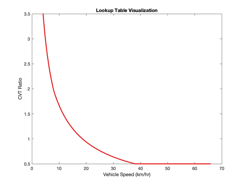
Hence, We can conclude that vehicle acceleration, deceleration and remains constant when the CVT Ratio is being varied.

Engine Speed Plot :

CVT Shaft Speed Plot :

Speed Vs. Throttle Plot :

5. BAJA ATV Model - Mapped Lookup Table With Dashboard (cvt Model dashboard mapped) :

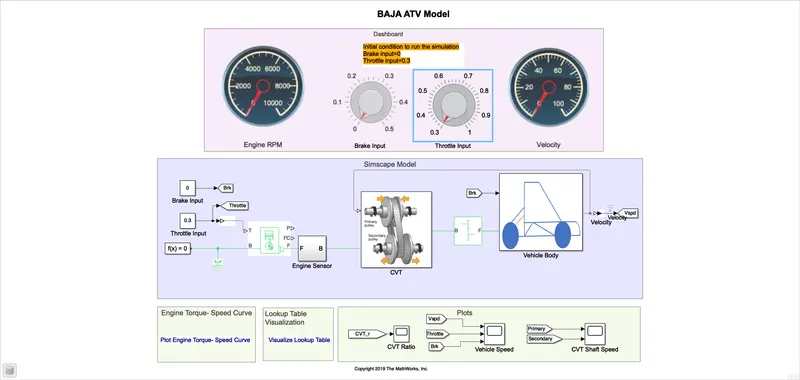
Main Model :

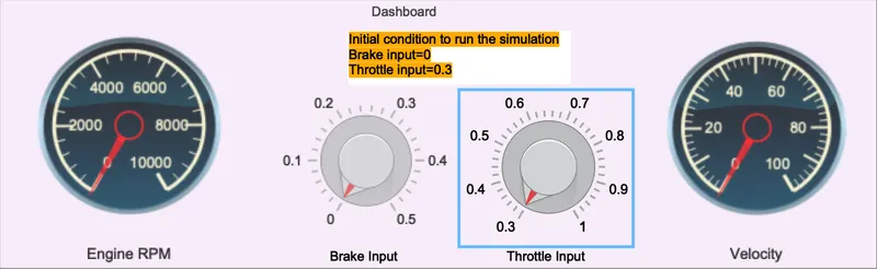
Dashboard (simulation OFF) :

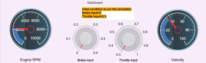
Dashboard (simulation ON) :

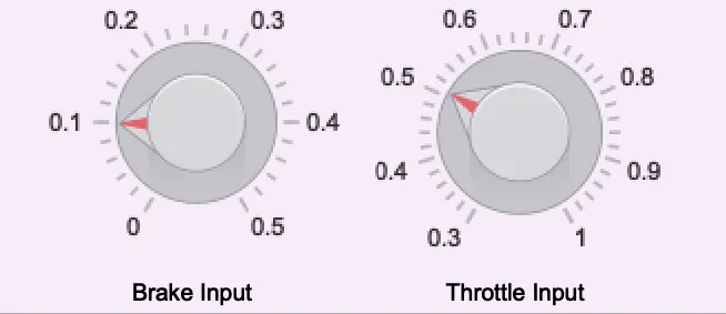
User Controller :

Explanation :

The Model workflow Process is same as process of " BAJA ATV model - Mapped Lookup Table without Dashboard ".

But Throttle and Brakes input are controlled by user with help of knobes followed by the vehicle speed is given as feed back to the CVT ratio lookup table.

CVT Ratio Plot :

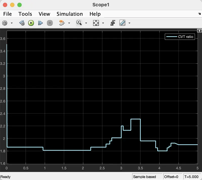
This BAJA ATV Model, The Engine is preset to run at 2400 rpm with Throttle Value at '0.3' and velocity at 40 KMPH. The CVT Ratio for minimum and maximum speed of the engine was pre-defined as 3.5 and 1.8 respectively. When Simulation is started initial throttle value 0.3 is achived so that CVT Ratio is nearly to 1.85. When Throttle value is being increased the CVT Ratio move towards 1.8 . Where the State is maximum engine speed. Simultaneously when throttle is being decreased CVT Ratio will move towards 1.85. While bracking is applied CVT Ratio increases so that it can achieve the nearest state of 3.5 (Minimum Engine speed). When braking is reduced the CVT Ratio moves towards 1.85 which is the basic throttle input 0.3 or if any other throttle value is applied it would reach that CVT Ratio state.

Engine Speed Plot :

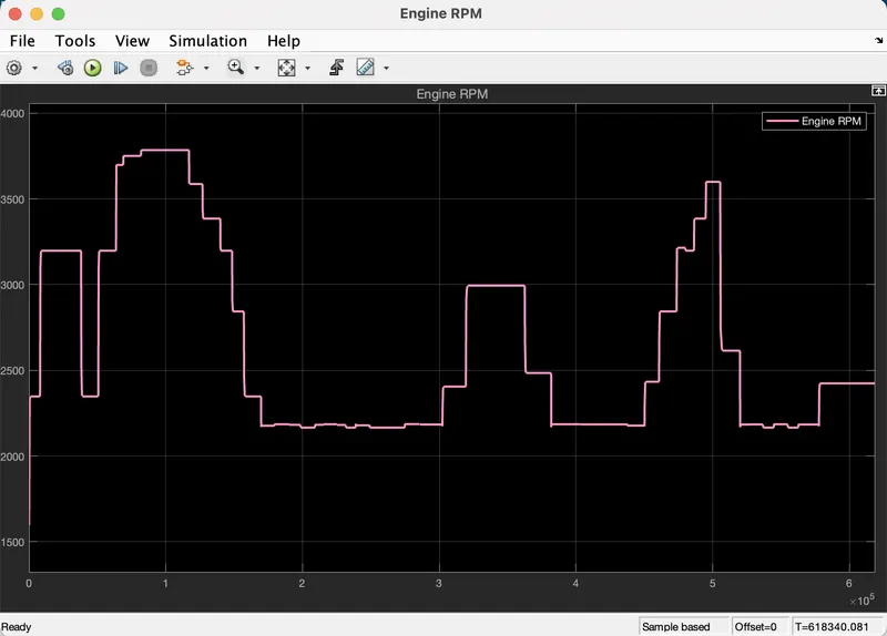
From graph we can take that vehicle was first running at Minimum RPM of 2400 RPM and When Throttle is Applied (Step-up) then Braking (Step-down). Then brake is released so that engine RPM is increased then braking is applied.

CVT Speed Reduction Plot :

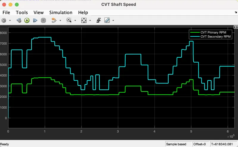
From above graph we can understand that throttle is applied (step-up) and then kept constant then braking is applied (step-down) then brake is released so that engine speed is increased with increased in throttle input.

Speed vs. THrottle Plot :

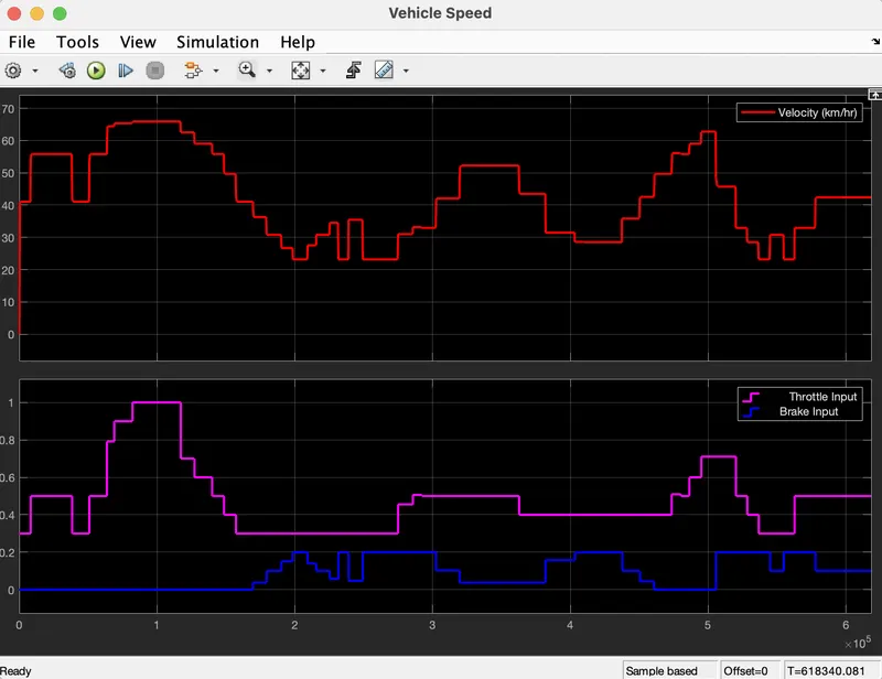
The Plot shows that we can read that when Throttle is applied the vehicle speed increases and when brake is applied vehicle speed decreases simultaneously.