Project

AIM :-

to study and analyse the baja all terrain vehicle(ATV) model using simulink and compare between different model

OBJECTIVES :-

• to prepare a technical report explaining the functions of the subsystems and blocks used for preparing the model
• to explain in detail all the differences between all the five models provided
• to understand and comment on the results

TYPES OF MODEL STUDIES :-

• BAJA ATV model without dashbord (cvt model)
• BAJA ATV model _ data extraction (cvt model data
• BAJA ATV model _ with dashbord (cvt model_dashbord)
• BAJA ATV model _ mapped lookup table without dashbord (cvt model_mapped)
• BAJA ATV model _ mapped lookup with dashbord (cvt model_dashbord_mapped)

INTRODUCTION :-

ALL TERRAIN VEHICLE

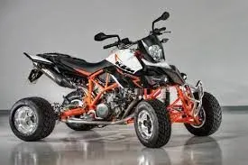
An all-terrain vehicle (ATV) is defined as a motorized off highway vehicle designed to travel on four low-pressure or non-pneumatic tires, having a seat designed to be straddled by the operator and handlebars for steering control. ATVs are subdivided into two types as designated by the manufacturer. Type I ATVs are intended by the manufacturer for use by a single operator and no passenger. Type II ATVs are intended by the manufacturer for use by an operator and a passenger, and are equipped with a designated seating position behind the operator.

BAJA SAE :-

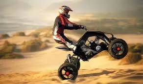
Baja SAE is an collegiate design series competition run by the Society of automotive engineers (SAE International). Teams of students from universities all over the world design and build small off-road cars. The cars all have. engines of the same specifications. As of 2018 the engine has been an unmodified briggs and stratton Model 19 Vanguard engine single cylinder with a displacement of 305cc and power output of approximately 10 bhp (7.5 kW).

The goal in Baja SAE racing is to design, build and race off road vehicles that can withstand the harshest elements of rough terrain. The vehicles used in Baja SAE racing are often similar in appearance to dune buggies. Before 2007, the events were called "Mini Baja

CONTINUOUSLY VARIABLE TRANSMISSION (CVT)

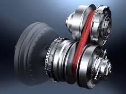
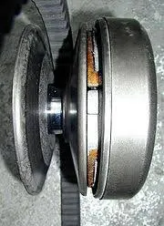
A continuously variable transmission (CVT) is anautomatic transmssion that can change seamlessly through a continuous range of gear ratios. This contrasts with other transmissions that provide a limited number of gear ratios in fixed steps. The flexibility of a CVT with suitable control may allow the engine to operate at a constant RPM while the vehicle moves at varying speeds.

MAIN AND CRITICAL BLOCKS USED :-

GENERIC ENGINE BLOCK :-

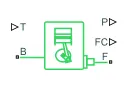
The Generic Engine block represents a general internal combustion engine. Engine types include spark-ignition and diesel Speed-power and speed-torque parameterizations are provided. A throttle physical signal input specifies the normalized engine torque. Optional dynamic parameters include crankshaft inertia and response time lag. A physical signal port outputs engine fuel consumption rate based on choice of fuel consumption model. Optional speed and redline controllers prevent engine stall and enable cruise control.

Main ports :-

1. B-Rotational Conserving Port representing the Engine Block(should be connected to rotational

motion reference)

2. F-Rotational Conserving Port representing the Engine Crankshaft
3. T-Physical signal input port :specifying the normalized engine throttle level
4. P- Physical signal output port: reporting the instantaneous engine power, in W
5. FC-Physical signal output port reporting the fuel consumption rate, in kg/s

SAMPLE GEAR :-

The Simple Gear block represents a gearbox that constrains the connected driveline axes of the base gear, B, and the follower gear, F. to corotate with a fixed ratio that is specified

The follower-base gear ratio is

gFB = rF/rB = NF/NB

where:

• Ngis the number of teeth in the base gear
• Ngfis the number of teeth in the follower gear

Main Ports :-

B-Base: Rotational mechanical conserving port associated with the base, or input shaft.

F-Follower: Rotational mechanical conserving port associated with the follower, or output, shaft

Variable Ratio Transmission block :-

The Variable Ratio Transmission block represents a gearbox that dynamically transfers motion and torque between the two connected driveshaft axes, base and follower.

Ignoring the dynamics of transmission compliance, the driveshafts are constrained to corotate with a Variable Gear Ratio control that you control. You can choose whether the follower axis rotates in the same or opposite direction as the base axis. If they rotate in the same direction, wF and wB have the same sign. If they rotate in opposite directions, we and why have opposite signs.

Transmission compliance introduces internal time delay between the axis motions. Therefore, unlike a gear, a variable transmission does not act as a kinematic constraint. You can also control torque loss caused by transmission and viscous losses.

MAIN PORTS :-

1.) B-Base Pulley or Drive Pulley

2.) F-Follower Pulley or Driven Pulley

3.) r-Variable Transmission Ratio (Input)

VEHICLE BODY BLOCK :-

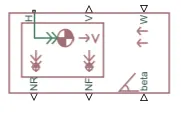
The Vehicle Body block represents a two-axle vehicle body in longitudinal motion. The vehicle can have the same or a different number of wheels on each axle. For example, two wheels on the front axle and one wheel on the rear axle. The vehicle wheels are assumed identical in size. The vehicle can also have a center of gravity (CG) that is at or below the plane of travel.

The block accounts for body mass, aerodynamic drag, road incline, and weight distribution between axles due to acceleration and road profile. Optionally include pitch and suspension dynamics. The vehicle does not move vertically relative to the ground.

The block has an option to include an externally-defined mass and an externally-defined inertia. The mass, inertia, and center of gravity of the vehicle body can vary over the course of simulation in response to system changes.

LIMITATIONS :-

The Vehicle Body block lets you model only longitudinali dynamics, parallel to the ground and oriented along the direction of motion. The vehicle is assumed to be in pitch and normal equilibrium. The block does not model pitch or vertical movement. As such, the equations assume that the wheels never lose contact. This constraint can result in negative normal forces.

INPUT PORTS :-

1.) Beta-Road Incline Angle (rad) physical signal input. port for road incline angle

2.) W-Head Wind Speed (m/s) physical signal input port for road incline angle

3.) CG-center of gravity(m) physical signal input port of externally defined mass relative to the cg of vehicle(only available with externally defined additional mass is set to on)

1.) M-mass(kg) physical signal input port for mass of the extemally defined mass(only available with externally defined additional mass is set to on)

2.) J-Externally defined moment of inertiain kg m 2) physical signal input port of the externally defined mass

OUTPUT PORTS :-

1.) NR-Rear Axle Normal Force (N): physical signal output port for the rear axle which is considered positive acting downward

2.) NF-Front Axle Normal Force (N) physical signal output port for the front axle which is considered positive acting downward

3.) V-Longitudinal Velocity (m/s) physical output signal of vehicle velocity

CONSERVING PORTS :-

H-Horizontal Motion: conserving port related to the horizontal motion of vehicle body(tyres should be i connected to this port)

DOUBLE SHOE BRAKE BLOCK :-

• The Double-Shoe Brake block represents a frictional brake with two pivoted rigid shoes that press against a rotating drum to produce a braking action. The rigid shoes sit inside or outside the rotating drum in a diametrically opposed configuration. A positive actuating force causes the rigid shoes to press against the rotating drum. Viscous and contact friction between the drum and the rigid shoe surfaces cause the rotating drum to decelerate.
• Double-shoe brakes provide high braking torque with small actuator deflections in applications that include motor vehicles and some heavy machinery. The model employs a simple parameterization with readily accessible brake geometry and friction parameters.

LIMITATIONS :-

• contact angles smaller than 45 degree produce less accurate results
• the brake uses the long shoe appoximation
• the brake geometry dose not self lock
• the model dose not account fpr actuator flow consumption

INPUT PORTS :-

F - physical signal input port associated with the applied actuating force

CONSERVING PORTS :-

S - rotational conserving port associated with the rotating drum shaft

TIRE(MAGIC FORMULA) BLOCK :-

The Tire (Magic Formula) block models a tire with longitudinal behavior given by the Magic Formula [1], an empirical equation based on four fitting coefficients. The block can model tire dynamics under constant or variable pavement conditions.

The longitudinal direction of the tire is the same as its direction of motion as it rolls on pavement. This block is a structural component based on the tire road interaction block.

To increase the fidelity of the tire model, you can specify properties such as tire compliance, inertia, and rolling resistance. However, these properties increase the complexity of the tire model and can slow down simulation. Consider ignoring tire compliance and inertia if simulating the model in real time or if preparing the model for hardware-in-the-loop (HIL) simulation.

EQUIVALENT MODEL :-

The full tire model is equivalent to this Simscape™/Simscape Driveline™ component diagram. It simulates both transient and steady-state behavior and correctly represents starting from, and coming to, a stop. The Translational Spring and Translational Damper are equivalent to the tire stiffness C_Fx and damping b_Fx. The Tire-Road Interaction (Magic Formula) block models the longitudinal force F_x on the tire as a function of F_z and k′ using the Magic Formula, with k′ as the independent slip variable.

The Wheel and Axle radius is the wheel radius r_w. The Mass value is the effective mass, Iwr2w. The tire characteristic function f(k′, F_z) determines the longitudinal force F_x. Together with the driveshaft torque applied to the wheel axis, F_x determines the wheel angular motion and longitudinal motion.

Without tire compliance, the Translational Spring and Translational Damper are omitted, and contact variables revert to wheel variables. In this case, the tire effectively has infinite stiffness, and port P of Wheel and Axle connects directly to port T of Tire-Road Interaction (Magic Formula).

Without tire inertia, the Mass is omitted.

LIMITATIONS :-

• The Tire (Magic Formula) block assumes longitudinal motion only and includes no camber, turning, or lateral motion.

• Tire compliance implies a time lag in the tire response to the forces on it. Time lag simulation increases model fidelity but reduces simulation performance.

INPUT PORTS :-

N - Normal force : Physical signal input port associated with the normal force acting on the tire. The normal force is positive if it acts downward on the tire, pressing it against the pavement.

M - Magic formula coefficients : Physical signal input port associated with the Magic Formula coefficients. Provide the Magic Formula coefficients as a four-element vector, specified in the order [B, C, D, E].

common tyre parameters :-

magic formula B coefficient :10

magic formula c coefficient : 1.9

magic formula D coefficient :1

magic formula E coefficient :0.97

OUTPUT PORTS :-

S - tire slip : physical signal output port associated with the relative slip between the tire and road

CONSERVING PORTS :-

A - axel : mechanical rotational port associated with the axle that the tire sits on

H - mechanical translational port associated with the wheel hub that transmits the thrust generated by the tire to the remoainder of the vehicle

OTHER BLOCKS USED :-

BAJA ATV MODEL WITHOUT DASHBORD (CVT MODEL)

MAIN MODEL :-

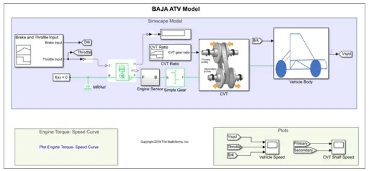
STEP :-

• The throttle signal is generated by signal builder block and inputted to generic engine.
• The torque and speed vector are inputted from the matlab workspace
• The engine will generate the output rpm which can be taken from the crankshaft output. This speed will be given to the Ideal Rotational Motion Sensor to sense the output rpm.
• The same output speed will be given to a simple gean mechanism to reduce the speed where the Gear Ratio is '4
• Then the output speed from the gear reducer will be given to the Variable Ratio Transmission block (CVT)
• The CVT ratio is provided to the Variable Ratio Transmission (CVT) block through Signal Builder.
• The speed is controlled by the variable CVT ratios and the controlled output speed is inputted to the vehicle axle
• The brake signal is generated by the signal builder and inputted to the vehicle body (Double Shoe Brake) for applying the brake to axle.
• The power from the CVT is inputted to the axle and the vehicle accelerates according to the speed.
• Then the Velocity is taken as output from the vehicle body for further analysis.

INPUT SIGNALS :-

THROTTLE INPUT SIGNAL :-

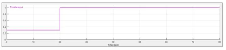
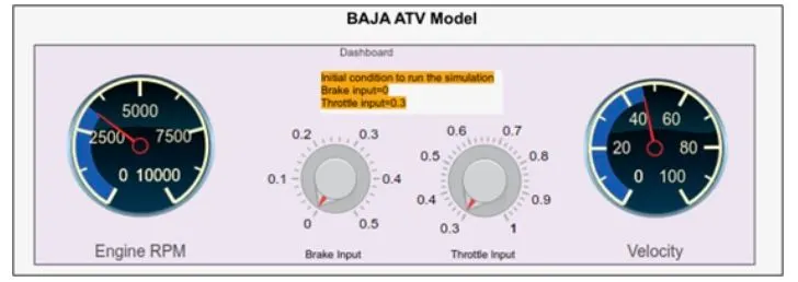
throttle starts at 0.3 and then it steps to 1 at the 20th second

BRAKE INPUT SIGNAL :-

the brake input remains zero through the whole simulation

TORQUE AND THE SPEED MATLAB WORKSPACE INPUT :-

CVT RATIO INPUT :-

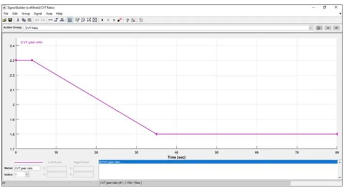
cvt ratio starts at 2.3 then 5 sec it gradually reduces until it reaches 1.8 at 35th sec and it remains so till the end of the simulation

ENGINE SENSOR SUB BLOCK :-

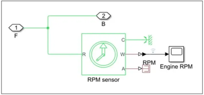
this subblock measure engine rotational speed as it takes the output of the engine as its input and output engine rpm

CVT SUB-BLOCK :-

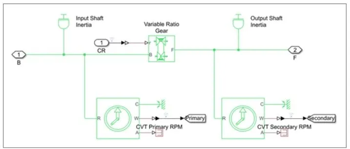
the cvt subblock provides the input and the output shafts of the cvt with inertia and measures the input shaft shaft rpm and the output shaft rpm

VEHICLE BODY SUB-BLOCK :-

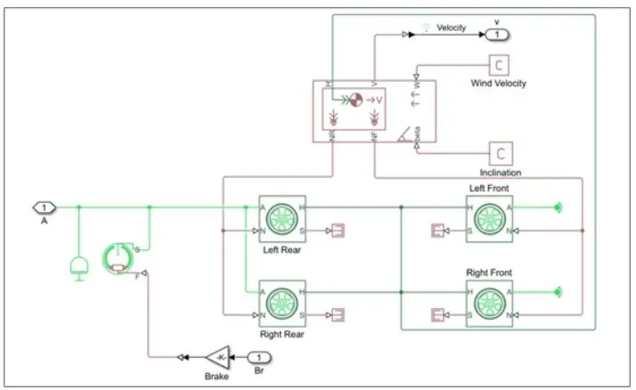
• The model shows that the vehicle is rear wheel drive as the output from the gearbox is inputted to the rear axle, then an inertia is added to simulate axle inertia, then the shoe brake s conserving port is connected to the axle, and then the same axle connects the two rear tyres while the front tyres is free to rotate on a rotational free end. All the tyres H hub port is connected together and then connected to the vehicle H port. Also the rear tyres N port is connected together and then connected to the vehicle body Nr output ports, while the front are connected to the Nf vehicle body output ports, the vehicle body takes the road inclination and wind velocity from physical constants.

RESULT :-

torque speed plot :-

the torque and the speed are inputted from the matlab workspace window to the generic engine block to generate the output rpm according this plot behavior is generic to all ICE

ENGINE SPEED PLOT :-

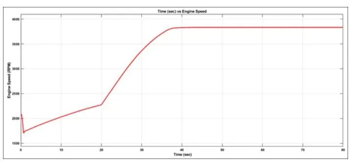
the engine rpm generated according to the throttle speed and torque input it is clearly evident how the step incress in throttle at 20th second resulted in an incress in the engine revolution from 2,250 to 3,800 rpm

ENGINE SPEED VS GEAR REDUCTION SPEED PLOT :-

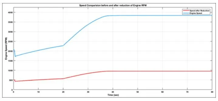
here we can see that the engine speed is reduced by the gear ratio '4'

maximum rpm (before reducing) = 3833 rpm was reduced to 958.25 rpm which can be varified by dividing the 3833 by the gear reduction ratio 4

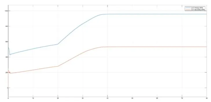
CVT SPEED REDUCTION PLOT :-

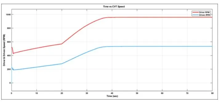
the engine reduced speed is controlled by various cvt ratios for verification the maximum rpm is calculated at 1.8 gear ratio which is applicable from the 35th second

maximum rpm (before reducing) = 958.25 rpm

CVT ratio = 1:1.8

gear ratio = driven/driver

1/1.8 = driven/958.25

driven = 958.25/1.8

driven = 532.36 rpm

the reduced maximum rpm is 532.36 rpm which can be verified from the plot

SPEED VS THROTTLE PLOT :-

From the graph we can infer that the brake is not applied during the drive cycle and the Throttle is constant (0.3) till 20 sec and being increased from 0.3 to 1 from 20 sec where it remains constant throughout. With increase in throttle the vehicle speed increased from 30 to 55 kmph.

BAJA AVT MODEL - DATA EXTRACTION (CVT MODEL - DATA)

MAIN MODEL :-

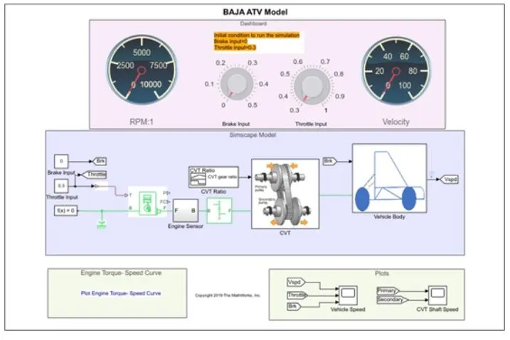
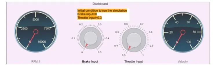
STEPS :-

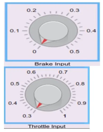
the model workflow process is same as the process of baja atv model without dashboard but the throttle and brake inputs are controlled by the user with knobs

RESULTS :-

ENGINE SPEED PLOT :-

here the engine speed is generated according to the inputs link throttle break torque and speed vectors the runtime is not defined so that the throttle and break are controlled by the user the step up is throttle and step down is breake input

ENGINE SPEED VS GEAR REDUCTION SPEED PLOT :-

the engine speed is reduced by a factor of 4 at any moment in the drive cycle as it is evident by the curve

CVT SPEED REDUCTION PLOT :-

the cvt gear reduction plot shows that at constant the reductiom ratio 1.8 is applicable at large time frame and it can be verified by taking 689 constant rpm and dividing it by 1.8 - 383 rpm which verifies the plot

SPEED VS THROTTLE INPUT :-

from the graph we can infer that the vehicle is accelerating while throttle is applied (step down) the constant speed areas represent no changes in throttle or braking

BAJA ATV MODEL - MAPPED LOOKUP TABLE WITHOUT DASHBOARD(CVT MODEL-MAPPED) :-

MAIN MODEL :-

STEPS :-

The model workflow process is same as the process of BAJA ATV model without Dashboard' except that it used instead of Signal Builder Blocks for Brake and Throttle Input Step input blocks are used. At 35 sec the brake input will take a step of value 'O' and at 20 sec throttle input will increases from 0.3-1 then remains constant throughout.

CVT SUB-BLOCK :-

• Interpolation is a process for estimating values that lie between known data points.
• Extrapolation is a process for estimating values that lie beyond the range of known data points.
• Rounding is a process for approximating a value by altering its digits according to a known rule.

RESULTS :-

CVT RATIO PLOT :-

When we compare the above plot, the ratio varies from 2.3 -1,8 within timespan of 80 sec which is same as the previous BAJA ATV Models. And from 32 sec it's constant ratio of 1.8' compared to 35 sec in the first model. Also the reduction from 2.3 ratio to 1.8 is not perfectly linear as in the first model.

CVT RATIO VS VEHICLE VELOCITY :-