Project 5

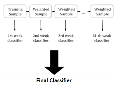
Boosting is an ensemble modeling technique that attempts to build a strong classifier from the number of weak classifiers. It is done by building a model by using weak models in series. Firstly, a model is built from the training data. Then the second model is built which tries to correct the errors present in the first model. This procedure is continued and models are added until either the complete training data set is predicted correctly or the maximum number of models are added.

AdaBoost was the first really successful boosting algorithm developed for the purpose of binary classification. AdaBoost is short for Adaptive Boosting and is a very popular boosting technique that combines multiple “weak classifiers” into a single “strong classifier”. It was formulated by Yoav Freund and Robert Schapire.

Algorithm:

1. Initialise the dataset and assign equal weight to each of the data point.
2. Provide this as input to the model and identify the wrongly classified data points.
3. Increase the weight of the wrongly classified data points.
4. if (got required results)
   Goto step 5
   else
   Goto step 2
   
5. End

Explanation:
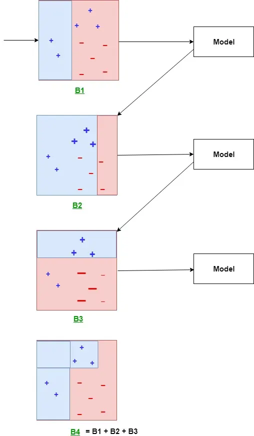
The above diagram explains the AdaBoost algorithm in a very simple way. Let’s try to understand it in a stepwise process:

• B1 consists of 10 data points which consist of two types namely plus(+) and minus(-) and 5 of which are plus(+) and the other 5 are minus(-) and each one has been assigned equal weight initially. The first model tries to classify the data points and generates a vertical separator line but it wrongly classifies 3 plus(+) as minus(-).
• B2 consists of the 10 data points from the previous model in which the 3 wrongly classified plus(+) are weighted more so that the current model tries more to classify these pluses(+) correctly. This model generates a vertical separator line that correctly classifies the previously wrongly classified pluses(+) but in this attempt, it wrongly classifies three minuses(-).
• B3 consists of the 10 data points from the previous model in which the 3 wrongly classified minus(-) are weighted more so that the current model tries more to classify these minuses(-) correctly. This model generates a horizontal separator line that correctly classifies the previously wrongly classified minuses(-).
• B4 combines together B1, B2, and B3 in order to build a strong prediction model which is much better than any individual model used.

Gradient Boosting is a popular boosting algorithm. In gradient boosting, each predictor corrects its predecessor’s error. In contrast to Adaboost, the weights of the training instances are not tweaked, instead, each predictor is trained using the residual errors of predecessor as labels.

There is a technique called the Gradient Boosted Trees whose base learner is CART (Classification and Regression Trees).

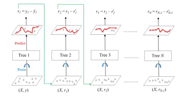
The below diagram explains how gradient boosted trees are trained for regression problems.

The ensemble consists of N trees. Tree1 is trained using the feature matrix X and the labels y. The predictions labelled y1(hat) are used to determine the training set residual errors r1. Tree2 is then trained using the feature matrix X and the residual errors r1 of Tree1 as labels. The predicted results r1(hat) are then used to determine the residual r2. The process is repeated until all the N trees forming the ensemble are trained.

There is an important parameter used in this technique known as Shrinkage.

Shrinkage refers to the fact that the prediction of each tree in the ensemble is shrunk after it is multiplied by the learning rate (eta) which ranges between 0 to 1. There is a trade-off between eta and number of estimators, decreasing learning rate needs to be compensated with increasing estimators in order to reach certain model performance. Since all trees are trained now, predictions can be made.

Each tree predicts a label and final prediction is given by the formula,

y(pred) = y1 + (eta *  r1) + (eta * r2) + ....... + (eta * rN)

The class of the gradient boosting regression in scikit-learn is GradientBoostingRegressor. A similar algorithm is used for classification known as GradientBoostingClassifier.

# Import models and utility functions
from sklearn.ensemble import GradientBoostingRegressor
from sklearn.model_selection import train_test_split
from sklearn.metrics import mean_squared_error as MSE
from sklearn import datasets
  
# Setting SEED for reproducibility
SEED = 1
  
# Importing the dataset 
bike = datasets.load_bike()
X, y = bike.data, bike.target
  
# Splitting dataset
train_X, test_X, train_y, test_y = train_test_split(X, y, test_size = 0.3, random_state = SEED)
  
# Instantiate Gradient Boosting Regressor
gbr = GradientBoostingRegressor(n_estimators = 200, max_depth = 1, random_state = SEED)
  
# Fit to training set
gbr.fit(train_X, train_y)
  
# Predict on test set
pred_y = gbr.predict(test_X)
  
# test set RMSE
test_rmse = MSE(test_y, pred_y) ** (1 / 2)
  
# Print rmse
print('RMSE test set: {:.2f}'.format(test_rmse))

• LightGBM (Light Gradient Boosting Machine)

LightGBM is a gradient boosting framework based on decision trees to increases the efficiency of the model and reduces memory usage.
It uses two novel techniques: Gradient-based One Side Sampling and Exclusive Feature Bundling (EFB) which fulfills the limitations of histogram-based algorithm that is primarily used in all GBDT (Gradient Boosting Decision Tree) frameworks. The two techniques of GOSS and EFB described below form the characteristics of LightGBM Algorithm. They comprise together to make the model work efficiently and provide it a cutting edge over other GBDT frameworks
Gradient-based One Side Sampling Technique for LightGBM:

Different data instances have varied roles in the computation of information gain. The instances with larger gradients(i.e., under-trained instances) will contribute more to the information gain. GOSS keeps those instances with large gradients (e.g., larger than a predefined threshold, or among the top percentiles), and only randomly drop those instances with small gradients to retain the accuracy of information gain estimation. This treatment can lead to a more accurate gain estimation than uniformly random sampling, with the same target sampling rate, especially when the value of information gain has a large range.
Algorithm for GOSS:

Input: I: training data, d: iterations
Input: a: sampling ratio of large gradient data
Input: b: sampling ratio of small gradient data
Input: loss: loss function, L: weak learner
models ? {}, fact ? (1-a)/b
topN ? a × len(I), randN ? b × len(I)
for i = 1 to d do
    preds ? models.predict(I) g ? loss(I, preds), w ? {1, 1, ...}
    sorted ? GetSortedIndices(abs(g))
    topSet ? sorted[1:topN]
    randSet ? RandomPick(sorted[topN:len(I)],
    randN)
    usedSet ? topSet + randSet
    w[randSet] × = fact . Assign weight f act to the

small gradient data.
    newModel ? L(I[usedSet], g[usedSet],
    w[usedSet])
    models.append(newModel)

according to the estimated variance gain at vector V_j (d) over the subset A ? B.

(1)

where A_l = {x_i ? A : x_ij ? d}, A_r = {x_i ? A : x_ij > d}, B_l = {x_i ? B : x_ij ? d}, B_r = {x_i ? B : x_ij > d}, and the coefficient (1-a)/b is used to normalize the sum of the gradients over B back to the size of A^c.

pip install lightgbm
 
# Importing Required Library
import pandas as pd
import lightgbm as lgb
 
# Similarly LGBMRegressor can also be imported for a regression model.
from lightgbm import LGBMClassifier
 
# Reading the train and test dataset
data = pd.read_csv("cancer_prediction.csv)
 
# Removing Columns not Required
data = data.drop(columns = ['Unnamed: 32'], axis = 1)
data = data.drop(columns = ['id'], axis = 1)
# Skipping Data Exploration
# Dummification of Diagnosis Column (1-Benign, 0-Malignant Cancer)
data['diagnosis']= pd.get_dummies(data['diagnosis'])
 
# Splitting Dataset in two parts
train = data[0:400]
test = data[400:568]
 
# Separating the independent and target variable on both data set
x_train = train.drop(columns =['diagnosis'], axis = 1)
y_train = train_data['diagnosis']
x_test = test_data.drop(columns =['diagnosis'], axis = 1)
y_test = test_data['diagnosis']
 
# Creating an object for model and fitting it on training data set
model = LGBMClassifier()
model.fit(x_train, y_train)
# Predicting the Target variable
pred = model.predict(x_test)
print(pred)
accuracy = model.score(x_test, y_test)
print(accuracy)

• XGBoost (eXtreme Gradient Boosting)

In this algorithm, decision trees are created in sequential form. Weights play an important role in XGBoost. Weights are assigned to all the independent variables which are then fed into the decision tree which predicts results. Weight of variables predicted wrong by the tree is increased and these the variables are then fed to the second decision tree. These individual classifiers/predictors then ensemble to give a strong and more precise model. It can work on regression, classification, ranking, and user-defined prediction problems.

XGBoost Features
The library is laser-focused on computational speed and model performance, as such, there are few frills.
Model Features
Three main forms of gradient boosting are supported:

• Gradient Boosting
• Stochastic Gradient Boosting
• Regularized Gradient Boosting

System Features

• For use of a range of computing environments this library provides-
• Parallelization of tree construction
• Distributed Computing for training very large models
• Cache Optimization of data structures and algorithm

# Importing the libraries
import numpy as np
import matplotlib.pyplot as plt
import pandas as pd
   
# Importing the dataset
dataset = pd.read_csv('Churn_Modelling.csv')
X = dataset.iloc[:, 3:13].values
y = dataset.iloc[:, 13].values
   
# Encoding categorical data
from sklearn.preprocessing import LabelEncoder, OneHotEncoder
labelencoder_X_1 = LabelEncoder()
  
X[:, 1] = labelencoder_X_1.fit_transform(X[:, 1])
labelencoder_X_2 = LabelEncoder()
X[:, 2] = labelencoder_X_2.fit_transform(X[:, 2])
onehotencoder = OneHotEncoder(categorical_features = [1])
  
X = onehotencoder.fit_transform(X).toarray()
X = X[:, 1:]
   
# Splitting the dataset into the Training set and Test set
from sklearn.model_selection import train_test_split
X_train, X_test, y_train, y_test = train_test_split(
        X, y, test_size = 0.2, random_state = 0)
  
# Fitting XGBoost to the training data
import xgboost as xgb
my_model = xgb.XGBClassifier()
my_model.fit(X_train, y_train)
   
# Predicting the Test set results
y_pred = my_model.predict(X_test)
# Making the Confusion Matrix
from sklearn.metrics import confusion_matrix
cm = confusion_matrix(y_test, y_pred)