Project 4

Let us consider a dataset where we have a value of response y for every feature x:

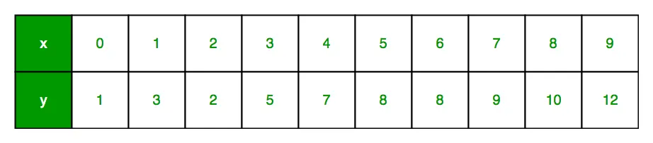
For generality, we define:
x as feature vector, i.e x = [x_1, x_2, …., x_n],
y as response vector, i.e y = [y_1, y_2, …., y_n]
for n observations (in above example, n=10).
A scatter plot of the above dataset looks like:-

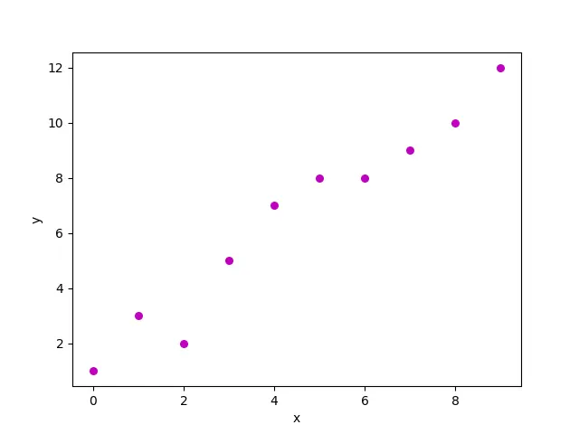
Now, the task is to find a line that fits best in the above scatter plot so that we can predict the response for any new feature values. (i.e a value of x not present in a dataset)
This line is called a regression line.
The equation of regression line is represented as:

Here,

• h(x_i) represents the predicted response value for i^th observation.
• b_0 and b_1 are regression coefficients and represent y-intercept and slope of regression line respectively.

To create our model, we must “learn” or estimate the values of regression coefficients b_0 and b_1. And once we’ve estimated these coefficients, we can use the model to predict responses!
In this article, we are going to use the principle of Least Squares.
Now consider:

Here, e_i is a residual error in ith observation.
So, our aim is to minimize the total residual error.
We define the squared error or cost function, J as:

and our task is to find the value of b_0 and b_1 for which J(b_0,b_1) is minimum!

Without going into the mathematical details, we present the result here:


where SS_xy is the sum of cross-deviations of y and x:

and SS_xx is the sum of squared deviations of x:

import numpy as np
import matplotlib.pyplot as plt
 
def estimate_coef(x, y):
    # number of observations/points
    n = np.size(x)
 
    # mean of x and y vector
    m_x = np.mean(x)
    m_y = np.mean(y)
 
    # calculating cross-deviation and deviation about x
    SS_xy = np.sum(y*x) - n*m_y*m_x
    SS_xx = np.sum(x*x) - n*m_x*m_x
 
    # calculating regression coefficients
b_1 = SS_xy / SS_xx
    b_0 = m_y - b_1*m_x
 
    return (b_0, b_1)
 
def plot_regression_line(x, y, b):
    # plotting the actual points as scatter plot
    plt.scatter(x, y, color = "m",
               marker = "o", s = 30)
 
    # predicted response vector
    y_pred = b[0] + b[1]*x
 
    # plotting the regression line
    plt.plot(x, y_pred, color = "g")
 
    # putting labels
    plt.xlabel('x')

plt.ylabel('y')
 
    # function to show plot
    plt.show()
 
def main():
    # observations / data
    x = np.array([0, 1, 2, 3, 4, 5, 6, 7, 8, 9])
    y = np.array([1, 3, 2, 5, 7, 8, 8, 9, 10, 12])
 
    # estimating coefficients
    b = estimate_coef(x, y)
    print("Estimated coefficients:\nb_0 = {}  \
          \nb_1 = {}".format(b[0], b[1]))
 
# plotting regression line
    plot_regression_line(x, y, b)
 
if __name__ == "__main__":
    main()

Bias
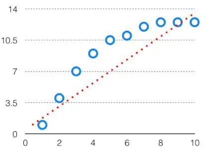
The bias is known as the difference between the prediction of the values by the ML model and the correct value. Being high in biasing gives a large error in training as well as testing data. Its recommended that an algorithm should always be low biased to avoid the problem of underfitting.
By high bias, the data predicted is in a straight line format, thus not fitting accurately in the data in the data set. Such fitting is known as Underfitting of Data. This happens when the hypothesis is too simple or linear in nature. Refer to the graph given below for an example of such a situation.

In such a problem, a hypothesis looks like follows.

Variance
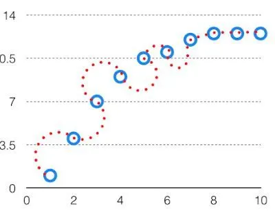
The variability of model prediction for a given data point which tells us spread of our data is called the variance of the model. The model with high variance has a very complex fit to the training data and thus is not able to fit accurately on the data which it hasn’t seen before. As a result, such models perform very well on training data but has high error rates on test data.
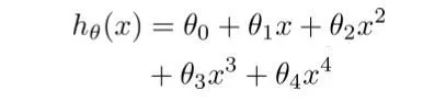
When a model is high on variance, it is then said to as Overfitting of Data. Overfitting is fitting the training set accurately via complex curve and high order hypothesis but is not the solution as the error with unseen data is high.
While training a data model variance should be kept low.

The high variance data looks like follows.

In such a problem, a hypothesis looks like follows.