Project 3
2.
- Gradient Descent
The work of the gradient descent algorithm is to update the weights in such a way that the loss function is minimum.
The updation rule is:
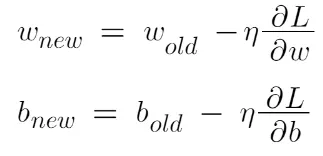
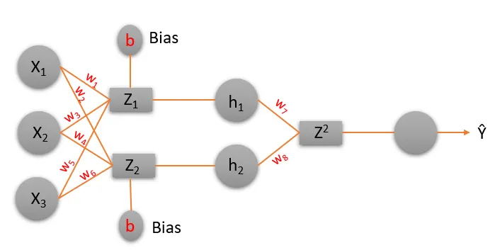
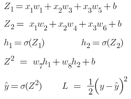
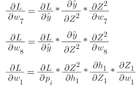
Now from the image above, we can calculate the values of Z1, Z2, etc, and all the derivates like in the images below.
Activation functions are used to introduce non-linearity.
Non-linearity in a neural network simply means a function that is able to classify the class of a function that is divided by a decision boundary that is not linear.
It is very hard to find any example in the real world which follows this linearity and hence we need some functions that can approximate a non-linear phenomenon.
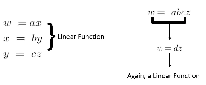
If we take all linear functions then the output is nothing but a constant multiplication by the input.
Similarly in a Neural Network, if we do not take non-linearity into account, then the output is just a summation.
of inputs and weights. No matter how many layers it had, our Neural Network would behave just like a single-layer perceptron.
Sigmoid Functions – The step activation function which is a logic used in perceptron is that if the value is greater than the threshold value then the output is 1 (neuron will fire) otherwise 0 (neuron will not fire) and this logic is used by perceptron is very harsh.
WHY SIGMOID?
Sigmoid functions are broadly used in Back Propagation Networks because of the relationship between the value of the function and the value of the derivative at that point. This reduces overall computation overload.
There are two types of sigmoidal functions:
- Binary Sigmoid
- Bipolar Sigmoid
Binary Sigmoid Function:
This is also known as logistic sigmoid function. Its range lies between 0 and 1. The Sigmoid function gives the output in probability and it is smoother than the perceptron function. If w(t)x tends to infinity then the output gets close to If w(t)x tends to negative infinity the output gets close to 0.
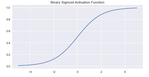
import numpy as np
import matplotlib.pyplot as plt
import numpy as np
plt.style.use('seaborn')
plt.figure(figsize=(8,4))
def SigmoidBinary(t):
    return 1/(1+np.exp(-t))
t = np.linspace(-5, 5)
plt.plot(t, SigmoidBinary(t))
plt.title('Binary Sigmoid Activation Function')
plt.show()
Bipolar Sigmoid Function: This is the function from where the Hyperbolic Tan Function was derived from. Here (lambda) represents the steepness factor. The range of this function is between -1 and 1. For the hyperbolic tangent function, the value of the steepness factor is 2.
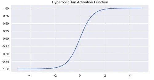
import numpy as np
import matplotlib.pyplot as plt
import numpy as np
plt.style.use('seaborn')
plt.figure(figsize=(8,4))
def HyperbolicTan(t):
    return np.tanh(t)
t = np.linspace(-5, 5)
plt.plot(t, HyperbolicTan(t))
plt.title('Hyperbolic Tan Activation Function')
plt.show()
1.
Gradient Descent is an iterative algorithm that is used to minimize a function by finding the optimal parameters. Gradient Descent can be applied to any dimension function i.e. 1-D, 2-D, 3-D. In this article, we will be working on finding global minima for parabolic function (2-D) and will be implementing gradient descent in python to find the optimal parameters for the linear regression equation (1-D). Before diving into the implementation part, let us make sure the set of parameters required to implement the gradient descent algorithm. To implement a gradient descent algorithm, we require a cost function that needs to be minimized, the number of iterations, a learning rate to determine the step size at each iteration while moving towards the minimum, partial derivates for weight & bias to update the parameters at each iteration, and a prediction function.
- Algorithm for Gradient Descent
Steps should be made in proportion to the negative of the function gradient (move away from the gradient) at the current point to find local minima. Gradient Ascent is the procedure for approaching a local maximum of a function by taking steps proportional to the positive of the gradient (moving towards the gradient).
repeat until convergence
{
    w = w - (learning_rate * (dJ/dw))
    b = b - (learning_rate * (dJ/db))
Step 1: Initializing all the necessary parameters and deriving the gradient function for the parabolic equation 4x2. The derivate of x2 is 2x, so the derivative of the parabolic equation 4x2 will be 8x.
x0 = 3 (random initialization of x)
learning_rate = 0.01 (to determine the step size while moving towards local minima)
gradient = (Calculating the gradient function)
Step 2: Let us perform 3 iterations of gradient descent:
For each iteration keep on updating the value of x based on the gradient descent formula.
Iteration 1:
    x1 = x0 - (learning_rate * gradient)
    x1 = 3 - (0.01 * (8 * 3))
    x1 = 3 - 0.24
    x1 = 2.76

Iteration 2:
    x2 = x1 - (learning_rate * gradient)
    x2 = 2.76 - (0.01 * (8 * 2.76))
x2 = 2.76 - 0.2208
    x2 = 2.5392

Iteration 3:
    x3 = x2 - (learning_rate * gradient)
    x3 = 2.5392 - (0.01 * (8 * 2.5392))
    x3 = 2.5392 - 0.203136
    x3 = 2.3360
# Importing Libraries
import numpy as np
import matplotlib.pyplot as plt

def mean_squared_error(y_true, y_predicted):

    # Calculating the loss or cost
    cost = np.sum((y_true-y_predicted)**2) / len(y_true)
    return cost

# Gradient Descent Function
# Here iterations, learning_rate, stopping_threshold
# are hyperparameters that can be tuned
def gradient_descent(x, y, iterations = 1000, learning_rate = 0.0001,
                     stopping_threshold = 1e-6):

    # Initializing weight, bias, learning rate and iterations
    current_weight = 0.1
current_bias = 0.01
    iterations = iterations
    learning_rate = learning_rate
    n = float(len(x))

    costs = []
    weights = []
    previous_cost = None

    # Estimation of optimal parameters
    for i in range(iterations):

        # Making predictions
        y_predicted = (current_weight * x) + current_bias

# Calculationg the current cost
        current_cost = mean_squared_error(y, y_predicted)

        # If the change in cost is less than or equal to
        # stopping_threshold we stop the gradient descent
        if previous_cost and abs(previous_cost-current_cost)<=stopping_threshold:
            break

        previous_cost = current_cost

        costs.append(current_cost)
        weights.append(current_weight)

        # Calculating the gradients
        weight_derivative = -(2/n) * sum(x * (y-y_predicted))
        bias_derivative = -(2/n) * sum(y-y_predicted)
# Updating weights and bias
        current_weight = current_weight - (learning_rate * weight_derivative)
        current_bias = current_bias - (learning_rate * bias_derivative)

        # Printing the parameters for each 1000th iteration
        print(f"Iteration {i+1}: Cost {current_cost}, Weight \
        {current_weight}, Bias {current_bias}")


    # Visualizing the weights and cost at for all iterations
    plt.figure(figsize = (8,6))
    plt.plot(weights, costs)
    plt.scatter(weights, costs, marker='o', color='red')
    plt.title("Cost vs Weights")
    plt.ylabel("Cost")
    plt.xlabel("Weight")
    plt.show()
return current_weight, current_bias


def main():

    # Data
    X = np.array([32.50234527, 53.42680403, 61.53035803, 47.47563963, 59.81320787,
           55.14218841, 52.21179669, 39.29956669, 48.10504169, 52.55001444,
           45.41973014, 54.35163488, 44.1640495 , 58.16847072, 56.72720806,
           48.95588857, 44.68719623, 60.29732685, 45.61864377, 38.81681754])
    Y = np.array([31.70700585, 68.77759598, 62.5623823 , 71.54663223, 87.23092513,
           78.21151827, 79.64197305, 59.17148932, 75.3312423 , 71.30087989,
           55.16567715, 82.47884676, 62.00892325, 75.39287043, 81.43619216,
           60.72360244, 82.89250373, 97.37989686, 48.84715332, 56.87721319])

# Estimating weight and bias using gradient descent
    estimated_weight, eatimated_bias = gradient_descent(X, Y, iterations=2000)
    print(f"Estimated Weight: {estimated_weight}\nEstimated Bias: {eatimated_bias}")

    # Making predictions using estimated parameters
    Y_pred = estimated_weight*X + eatimated_bias

    # Plotting the regression line
    plt.figure(figsize = (8,6))
    plt.scatter(X, Y, marker='o', color='red')
    plt.plot([min(X), max(X)], [min(Y_pred), max(Y_pred)], color='blue',markerfacecolor='red',
             markersize=10,linestyle='dashed')
    plt.xlabel("X")
    plt.ylabel("Y")
    plt.show()