Project 2 - Speed Control of a Direct Current (DC) motor

Develop a mathematical model of the DC motor, and a controller (PID) to achieve the desired speed (x1_ref).

1. Mathematics Modelling:

In a DC motor, we have two circuits:

1. Field Circuit

2. Armature / Rotor Circuit.

The objective of the motor is to generate required speed and torque on the rotor.

Principle of working:

> Rotor a current carrying conductor, when placed in a magnetic field, generated by the current flow in field circuit, experiences a mechanical force.

> These forces generate torque on the rotor. And the direction of the rotation is based on the Fleming's left-hand rule.

The equations related to field circuit:

Vf = Rf * If + Lf * d(If)/dt --> (Kirchoff's voltage law) --- Eqn (1)

where,

Vf = Field Voltage (volts)

Rf = Field Resistance (ohms)

Lf = Field Inductance (henry)

If = Field Current (amps)

assuming steady state current flow in field circuit

d(If)/dt = 0;

Therefore, If = Vf/Rf --- Eqn (2)

The equations related to armature circuit:

Vs = Ra * Ia + La * d(Ia)/dt + Vb; (kirchoff's voltage law) --- Eqn (3)

where,

Vs = supply voltage to rotor / armature (volts)

Ra = Armature resistance (ohms)

La = Armature inductance (henry)

Vb = Back Emf - Induced (volts)

Ia = Armature Current (amps)

Vb = ke*w; --- Eqn (4)

where,

w = speed (rad/s)

ke = Back Emf constant = km* phi (v*s/rad) --- Eqn (5)

km = motor constant (v*s/(rad*wb))

phi = magnetic field flux = k_phi * If (Wb) --- Eqn (6)

K_phi = proportionality constant (Wb/A)

Therefore, Vb = km*k_phi*If*w --- Eqn (7)

Relation between Torque, Current and Speed.

T = K_t * Ia (N*m) --- Eqn (8)

T = J*dw/dt + Bm*w (N*m) --- Eqn (9)

where,

k_t = torque constant (N*m/A)

J = Polar moment of Inertia (kg *m^2)

Bm = Damping due to friction (N*m-s/rad)

So, the parameters needed for modeling of a DC motor are:

Vf, Rf, Ra, La, km, K_phi, K_t, w, J and Bm

Modelling the open loop transfer function (in S domain - Laplace transformed) from the above equation

>> Input = Vs (Supply voltage)

>> Output = w (Speed)

From Eqn (8) and (9)

k_t * Ia = J*dw/dt + Bm*w

Applying Laplace transform: k_t * Ia = J*w*s + Bm*w

since, w(t)

Rewrite interms of Ia: Ia = [(J*s + Bm) * w]/k_t --- Eqn (10)

Applying Laplace transfrom to Eqn (3): Vs = Ra*Ia + La*Ia*s + Vb --- Eqn (11)

since, Ia(t)

substitute Eqn (7) in Eqn (11), then

Vs = Ra*Ia + La*Ia*s + km*k_phi*If*w --- Eqn (12)

Substitute Eqn (10) in Eqn (12)

Vs = [(Ra + La*s) * (J*s + Bm)*w/k_t ] + km * k_phi * If * w

Re-arranging the terms

Vs = w * [(Ra + La*s) * (J*s + Bm) + k_t * km * k_phi * If] / k_t

Converting to Open loop transfer function

w / Vs = k_t / [(Ra + La*s) * (J*s + Bm) + k_t * km * k_phi * If]

2. Modelling the Electrical Engineering System in Matlab

% DC Motor model

3. Simulink Modeling

In designing a controller, we need to define the input & output parameters

In the DC motor, - speed control design, the parameters derived from the transfer function.

Control Parameter:

> Supply Voltage (Vs)

Vs = Kp * (X1ref - X1) - Kd*X2 + Ki*int(X1ref-x1)

X1 = W

X2 = Ia (Armature Current)

Reference Parameter

X1ref = W1ref (Reference Speed)

Output Parameter

X1 = W

The controller targets are:

(i) Setting Time: < 2 seconds

(ii) Overshoot : < 10%

(iii) SSE: <2%

The simulink model is developed, in such a way, we can able to extract the Armature Current (Ia), Torque (T) and Back EMF (Vb)

Re-arranging the Eqn (12),

w = (Vs - Vb)*K_t/[(La*s + Ra)*(J*s + Bm)

where,

Armature Current (Ia) = (Vs - Vb) / (La*s + Ra)

Torque (T) = Armature Current (Ia) * K_t

<Included in the above equation>

Back EMF volt (Vb) = w*k_m*k_phi*If

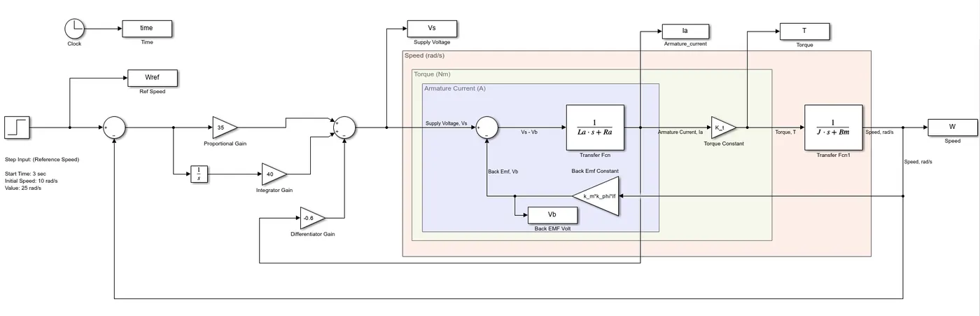
The input Speed-ref is defined as below:

Step Input (reference Speed)

Start Time: 3 sec

Initial: 10 rad/s

final: 25 rad/s

Iteration 1:

for Zeta = 0.5 - controller damping factor

Kp = 38.3133

Kd = -2.8584

>> Ki = 25 <<

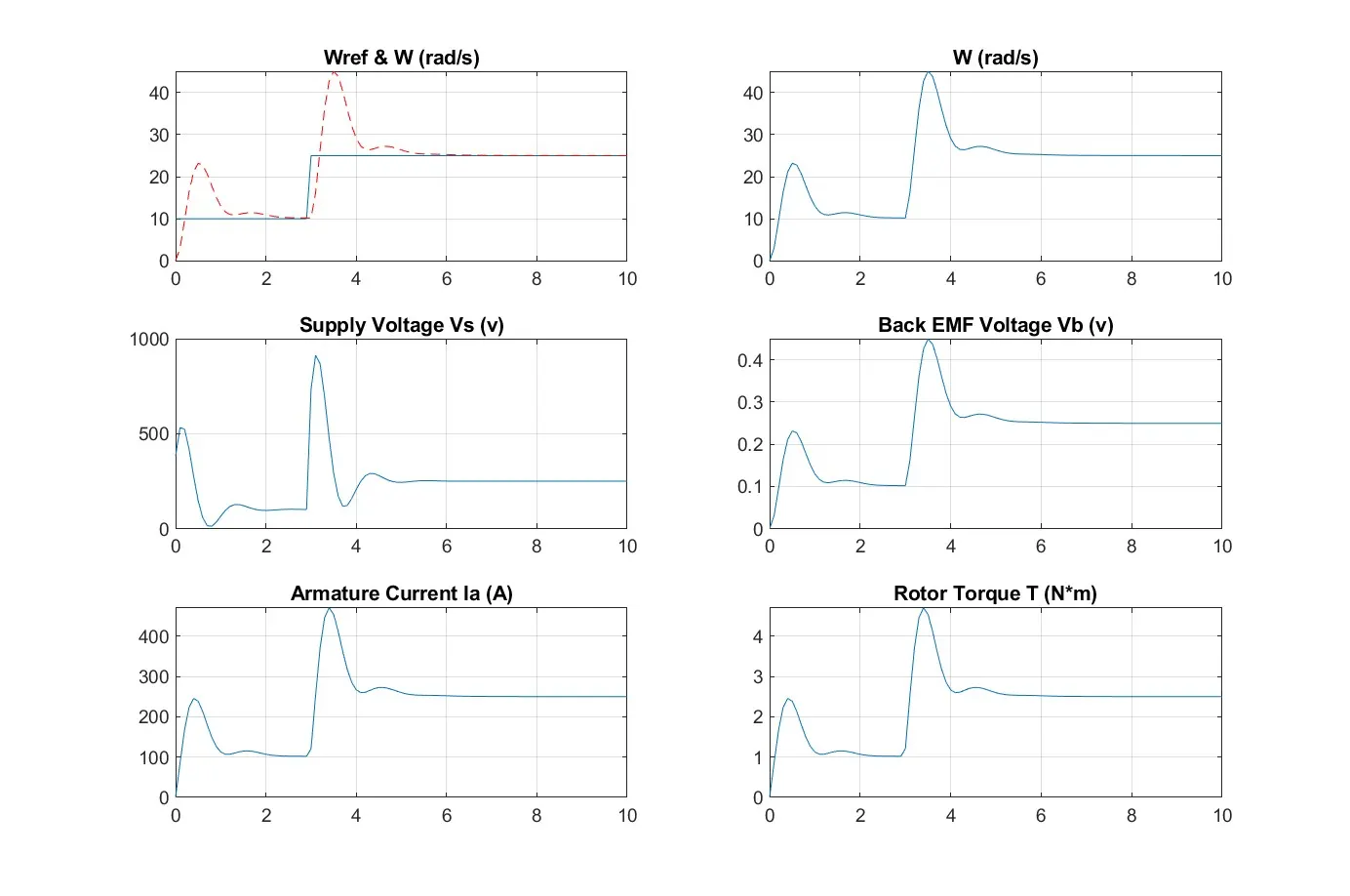
We can observe that the system reaches stable, but the overshoot seems high.

Iteration 2:

Increase the damping, zeta = 0.7 and keeping the Ki = 25

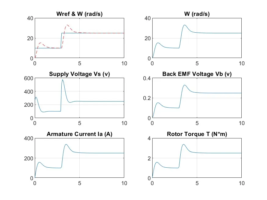
We can observe the increase in stability, and reduction in overshoot, but it is still >50 % of the reference speed.

Iteration 3:

The values of controller were tuned to

Kp = 35;

kd = -1.6018 (zeta = 0.7)

Ki = 40

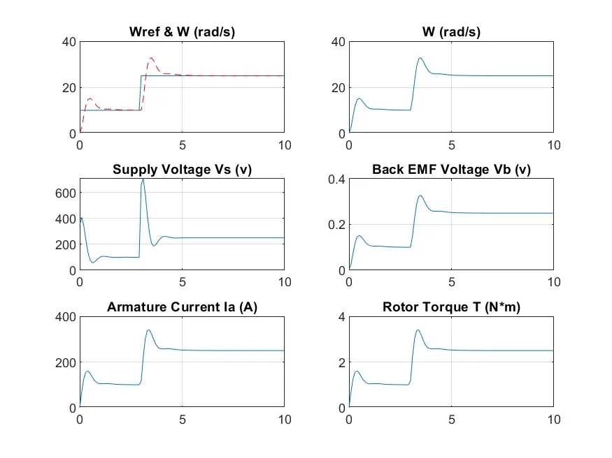
Iteration 4:

The values of controller were tuned to

Kp = 25.7469;

kd = -0.6

Ki = 40

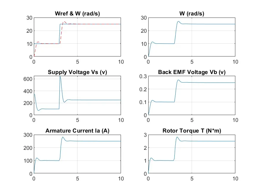
For the above value, it is witnessed that we are able to control the stabilize the motor, even the speed is changed.

Also, the overshoot, settling time and SSE are well under the target values.

Summary:

We explored the working principle and the mathematical modeling of a DC motor. The same was implemented in the MATLAB script and exported to the simulink model with a PID controller. The model was tested with various combinations of the proportional, integral and derivative gains. From the simulation results, it was observed that increasing the proportional gain enhances the speed of the response (iteration 3 & 4), the derivative gain reduces the oscillations and improve the stability, while the integral gain effectively minimizes the steady-state error.