Project 2 - Rankine cycle Simulator
Simulating ideal rankine cycle in MATLAB:
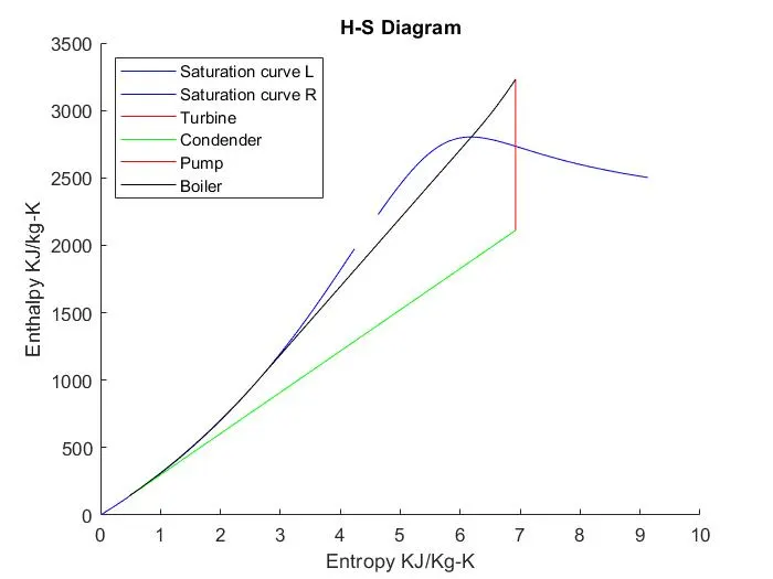
The aim of this project is to simulate the working of ideal rankine cycle and plot the T-S and H-S graphs and print the values of the state point variables in the command window.
Objective:
The objective is to calculate Net work ratio and Back work ratio.
Rankine Cycle:
The Rankine cycle or Rankine Vapor Cycle is the process widely used by power plants such as coal-fired power plants or nuclear reactors. In this mechanism, a fuel is used to produce heat within a boiler, converting water into steam which then expands through a turbine producing useful work.
The various components involved in the ideal rankine cycle are:
Pump: Compression of the fluid to high pressure using a pump (this takes work)
Boiler: The compressed fluid is heated to the final temperature (which is at boiling point), therefore, a phase change occurs—from liquid to vapor
Turbine: Expansion of the vapor in the turbine.
Condenser: Condensation of the vapor in the condenser (where the waste heat goes to the final heat sink (the atmosphere or a large body of water (ex. lake or river).
Formulae:
Net work ratio= (Net work)/(Heat supplied)
Back work ratio= (Work consumed by pump)/(Work produced by turbine)
The program used for solving this was MATLAB.
MATLAB code:
% Rankine cycle simulator - A program that calculates the results on all
% the state points based on the given inputs and plots the P-V and T-S
% diagram of a rankine cycle

clear all
close all
clc

% Acquiring essential inputs
disp('Rankine Cycle Simulator')
disp('1-2 corresponds to isentropic expansion in turbine')
disp('2-3 corresponds to constant pressure heat rejection in condenser')
disp('3-4 corresponds to isentropic compression in pump')
disp('4-1 corresponds to constant pressure heat addition in boiler')
fprintf('\n')

p1=input('Enter the pressure at the inlet of turbine (bar)=    ');
t1=input('Enter the temp at the inlet of turbine (degree C)=    ');
p2=input('Enter the pressure at the inlet of condenser (bar)=   ');

% At state point 1
h1=XSteam('h_pt',p1,t1);
s1=XSteam('s_pt',p1,t1);

% At state point 1
% Since 1-2 is isentropic
s2=s1;

sf2=XSteam('sL_p',p2);
sg2=XSteam('sV_p',p2);
sfg2=(sg2-sf2);

% Finding dryness fraction (s2 = sf2 + x2 * sfg2)

x2=(s2-sf2)/sfg2;

if x2<1;
    disp('Steam is wet at the inlet of the condenser')
    fprintf('\n')

    % Finding enthaly

    hf2=XSteam('hL_p',p2);
    hg2=XSteam('hV_p',p2);
    hfg2=hg2-hf2;
    h2=hf2+x2*hfg2;

    t2=XSteam('Tsat_p',p2);

    % Work done by turbine
    wt=h1-h2;


    % For state point 3
    %Work done by pump
    p3=p2;
    vf3=XSteam('vL_P',p3);
    v3=vf3;
    wp=v3*(p1-p2)*100;
    t3=XSteam('Tsat_p',p2);
    h3=XSteam('hL_p',p2);
    s3=XSteam('sL_p',p2);

    % At state point 4
    p4=p1;
    h4=wp+h3;
    t4=XSteam('T_ph',p4,h4);
    s4=s3;
    % Heat supplied to boiler
    qs=h1-h4;

    % Heat rejected by condenser
    qr=h2-h3;

    % Work ratios and effeciecny of turbine
    w_net=wt-wp;


    net_work_ratio=w_net/wt;
    effeciency=w_net/qs;

    % Back work ratio
    back_work_ratio=wp/wt;

    % Specific steam consumption
    SSC=3600/w_net;
    tf_sat=XSteam('Tsat_p',p1);
    sf_sat=XSteam('sL_p',p1);
    hf_sat=XSteam('hL_p',p1);
    sg_sat=XSteam('sV_p',p1);
    hg_sat=XSteam('hV_p',p1);

    % Plotting saturation liquid and vapour lines

    temp_range = linspace(1, 373, 1000);
    for i = 1 : length(temp_range)
            S_L(i) = XSteam('sL_T', temp_range(i));
            S_V(i) = XSteam('sV_T', temp_range(i));
    end


    % Plotting T-S diagram
    figure(1)
    hold on
    plot(S_L,temp_range,'b')
    plot(S_V,temp_range,'b')
    plot([s1 s2], [t1 t2],'r')
    plot([s2 s3], [t2 t3],'g')
    plot([s3 s4], [t3 t4],'b')

    % Plotting curved constant pressure line from 3 to 4
    t_cons_p=linspace(t4,XSteam('Tsat_p',p1),30);
    for i=1:length(t_cons_p);
        S(i)=XSteam('s_pt',p1 ,t_cons_p(i));

    end

    plot(S,t_cons_p,'k')

    t0_cons_p=linspace(XSteam('Tsat_p',p1),t1,300);

    for i=1:length(t0_cons_p);
        S0(i)=XSteam('s_pt',p1 ,t0_cons_p(i));

    end

    plot(S0,t0_cons_p,'k')

    % Plotting the straight line of the phase change region
    plot([sf_sat sg_sat],[tf_sat tf_sat],'k')

    title('T-S Diagram')
    xlabel('Entropy KJ/Kg-K')
    ylabel('Temperature degreee C')
    axis([0 10 0 700])

    legend('Saturation curve L','Saturation curve R','Turbine','Condender','Pump','Boiler','location','northwest')


    % Plotting H-S diagram

    figure(2)
    hold on

    % Plotting saturation curves

    temp_range1 = linspace(1, 373, 1000);
    for i = 1 : length(temp_range1)
            H_L1(i) = XSteam('hL_T', temp_range1(i));
            H_V1(i) = XSteam('hV_T', temp_range1(i));

    end


     plot(S_L,H_L1,'b')
     plot(S_V,H_V1,'b')

     plot([s1 s2],[h1 h2],'r')
     plot([s2 s3],[h2 h3],'g')
     plot([s3 s4],[h3 h4],'r')

     % For plotting the line between the pump and boiler
     s_pump=linspace(s3,s1,1000);
     for i=1:length(s_pump)
            h_pump(i)=XSteam('h_ps',p1,s_pump(i));
     end


     plot(s_pump,h_pump,'k')

     title('H-S Diagram')
     xlabel('Entropy KJ/Kg-K')
     ylabel('Enthalpy KJ/kg-K')
     legend('Saturation curve L','Saturation curve R','Turbine','Condender','Pump','Boiler','location','northwest')

     % Displaying the value of state point variables at each point

     P_final=[p1 p2 p3 p4];
     T_final=[t1 t2 t3 t4];
     H_final=[h1 h2 h3 h4];
     S_final=[s1 s2 s3 s4];


     for i=1:4;
         fprintf('At state point %d \n',i)
         fprintf('Pressure p%d     :  %4.4f  (bar) \n',i,P_final(i))
         fprintf('Temperature t%d  :  %4.4f  (degree C) \n',i,T_final(i))
         fprintf('Enthalpy h%d     :  %4.4f (KJ/kg-K)\n',i,H_final(i))
         fprintf('Entropy s%d      :  %4.4f   (KJ/kg-K)\n',i,S_final(i))
         fprintf('\n')
     end

      fprintf('The net work ratio is: %f \n',net_work_ratio)
      fprintf('The back work ratio is: %f \n',back_work_ratio)


else
         fprintf('The entered values are not vaild as the steam is either Saturated or Super-saturated at the inlet of the condenser \n')
         fprintf('Enter the valid values by running the program again \n')
         return;
end
Explanation for the code:
1. The known inputs are collected initially using the input command (p1,t1 and p2).
2. Using the relations between the various properties of the ideal rankine cycle the values are calculated for all the state points.
3. In order to obtain the values from the steam table, the function XSteam is added to the current working folder of MATLAB. Using the appropriate input parameters for the XSteam function, the required values can be obtained.
4. The if statement is used to check if the dryness fraction falls within the wet, dry-saturated or the super heated range.
5. Once the state point variables are calculated, the net work ratio and back work ratio can be calculated.
6. Plot command is then used to obtain TS and HS diagram.
7. Finally fprintf command is used to display all the values of the state point variables in the command window.
Input values:
p1=30 bar
t1=400 degree C
p2=0.05 bar
Results:
1. Temperature-entropy diagram
2.Enthalpy-Entropy diagram
3. Command window
Conclusion:
Thus the net work ratio and back work ratio for ideal rankine cycle was calculated using MATLAB.
1. Net work ratio = 0.997314
2. Back work ratio = 0.002686
Referenes:
1. https://www.youtube.com/watch?v=Ec9kXfrZaR4&list=PLwdnzlV3ogoV0lD0LHaprmm0sRHIOANe6&index=3
3. http://twt.mpei.ac.ru/TTHB/2/KiSyShe/eng/Chapter11/11-2-The-Rankine-cycle.html
4. Natarajan.E, Engineering Thermodynamics: Fundamentals and applications