Project 2 - Rankine cycle Simulator

Understand the concept of Rankine cycle by referring to standard thermal engineering text book.

• Create a Rankine Cycle Simulator using OCTAVE/MATLAB.
• Your code should calculate the state points of the Rankine Cycle (any type of your choice) based on user inputs.
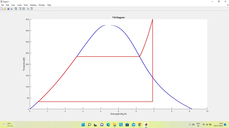
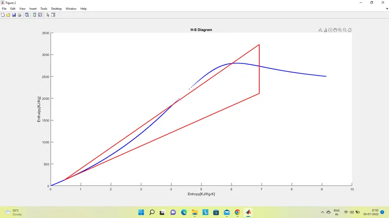
• Then, plot the corresponding T-s and h-s plots for the given set of inputs. Title and axes labels are a must, while legends could be used if necessary.
• The presentation of your code will be taken into consideration while grading. Labelling sections of your code using comments is appreciated.
• Attach a report explaining the working of a rankine cycle simulator and also the research done by you.

Contents expected in the report:

• Step-wise explanation of your code.
• Mention the errors faced while programming.
• Steps taken to overcome those errors.
• Screenshots showing errors thrown in command window.

The link for the standard Xsteam library to get the steam table data for water, is given below. It must be used to calculate the points in between the state variables.

Click here to download the Xsteam Library.

Required Inputs:

Turbine Inlet temperature = 400° C

Turbine Inlet Pressure = 30 bars

Turbine Outlet Pressure = 0.05 bars = Condenser Inlet Pressure

Calculate the followings,

• Net work output
• Back work ratio

Hints:

1.Code the basic program that calculates the state points alone

2.Then add the thermodynamic relation to get the points inbetween the state variables.

Sample output of a Basic Rankine cycle simulator:

• Type:Basic Rankine-

• Code Snippet -

• Output Screen -

clear
clc
%Process Information
fprintf('Rankine Cycle Simulator n')
fprintf('process 1-2 : Isentropic Expansion n')
fprintf('process 2-3 : Isobaric Heat Rejection n')
fprintf('process 3-4 : Isentropic compression n')
fprintf('process 4-1 : Isobaric heat addition process n')

%Initial Inputs
P1 = input('Enter the inlet pressure of Turbine: ');
P2 = input('Enter the outlet pressure from Turbine: ');
T1 = input('Enter the steam inlet Temperature: ');

%State point 1
H1 = XSteam('h_pT',P1,T1); %Enthalpy
S1 = XSteam('s_pT',P1,T1); %Entropy
Hf1 = XSteam('hL_p',P1); %Enthalpy of saturated liquid
Hg1 = XSteam('hV_p',P1); %Enthalpy of saturated vapour
Ts1 = XSteam('Tsat_P',P1); %Saturation Temp
Sf1 = XSteam('sL_p',P1); %Entropy of saturated liquid
Sg1 = XSteam('sV_p',P1); %Entropy of saturated vapour

%State point 2
S2 = S1;
Sf2 = XSteam('sL_p',P2);
Sg2 = XSteam('sV_p',P2);
Hf2 = XSteam('hL_p',P2);
Hg2 = XSteam('hV_p',P2);
x = (S2-Sf2)/(Sg2-Sf2); %Dryness Fraction
H2 =Hf2+x*(Hg2-Hf2);
T2 = XSteam('T_ph',P2,H2);
Ts2= XSteam('Tsat_p',P2);

%State Point 3
H3 = Hf2;
S3 = Sf2;
T3 = T2;
P3 = P2;

%State point 4
P4 = P1;
S4 = S3;
H4 = XSteam('h_ps',P4,S4);
T4 = XSteam('T_Ps',P4,S4);

t = linspace(0,374,500);

%Plot T-S Diagram
figure(1)
hold on

for i = 1:length(t)
plot(XSteam('sL_T',t(i)),t(i),'.','color','b')
plot(XSteam('sV_T',t(i)),t(i),'.','color','b')
end

%Plot Cycle,
plot([S1,S2],[T1 T2],'linewidth',2,'color','r')
if x>1
T3 =Ts2;
plot([S2 Sg2 S3 S4],[T2,Ts2 T3 T4],'linewidth',2,'color','r')
T2 = Ts2;
else
plot([S2 S3 S4],[T2 T3 T4],'linewidth',2,'color','r');
end

l = linspace(T1,T2,1000);

for i=1:length(l)
plot(XSteam('s_pT',P1,l(i)),l(i),'.','color','r')
end
plot([Sf1 Sg1],[Ts1 Ts1],'linewidth',2,'color','r')
xlabel('Entropy[KJ/Kg-K]')
ylabel('Temprature[K]')
title('T-S Diagram')

%Plot H-S Diagram
figure(2)
hold on

%Plot Saturation Curve
for i=1:length(t)
plot(XSteam('sL_T',t(i)),XSteam('hL_T',t(i)),'.','color','b')
plot(XSteam('sV_T',t(i)),XSteam('hV_T',t(i)),'.','color','b')
end

%Plot Cycle
plot([S1 S2 S3 S4 S1],[H1 H2 H3 H4 H1],'linewidth',2,'color','r')
xlabel('Entropy[KJ/Kg-K]')
ylabel('Enthalpy[KJ/Kg]')
title('H-S Diagram')

%calcualtion

%Turbine Work
wt = H1-H2;

%Pump Work
wp = H4-H3;

%Heat Addistion
Qin = H1-H4;

%Heat Rejection
Qout = H2-H3;

%Net Work
Wnet=wt-wp;

%Efficiency
Ntherm = (Wnet/Qin)*100;

%Specific stem consumption
SSC = 3600/Wnet;

%Back power Ratio
BWR= wp/wt;

%Print Result
fprintf('nnResultsn')
fprintf('At State Point 1:n')
fprintf('P1 is : %.2f barn',P1)
fprintf('T1 is : %.2f Deg Celciusn',T1)
fprintf('H1 is : %.2f KJ/Kgn',H1)
fprintf('S1 is : %.2f KJ/Kg-Kn',S1)

fprintf('nAt State Point 2:n')
fprintf('P2 is : %.2f barn',P2)
fprintf('T2 is : %.2f Deg Celciusn',T2)
fprintf('H2 is : %.2f KJ/Kgn',H2)
fprintf('S2 is : %.2f KJ/Kg-Kn',S2)

fprintf('nAt State Point 3:n')
fprintf('P3 is : %.2f barn',P3)
fprintf('T3 is : %.2f Deg Celciusn',T3)
fprintf('H3 is : %.2f KJ/Kgn',H3)
fprintf('S3 is : %.2f KJ/Kg-Kn',S3)

fprintf('nAt State Point 4:n')
fprintf('P4 is : %.2f barn',P4)
fprintf('T4 is : %.2f Deg Celciusn',T4)
fprintf('H4 is : %.2f KJ/Kgn',H4)
fprintf('S4 is : %.2f KJ/Kg-Kn',S4)

fprintf('nWt is : %.2f KJ/Kgn',wt)
fprintf('Wp is : %.2f KJ/Kgn',wp)
fprintf('Wnet is : %.2f KJ/Kgn', Wnet)
fprintf('Thermal Efficiency is : %.2f percentn',Ntherm)
fprintf('S.S.C. is : %.2f Kg/KWhn',SSC)
fprintf('Back Work Ratio is : %.3f n',BWR)

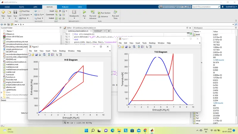
1. Xsteam data is used to extract steam and water properties of enthaly , entropy at specific pressure and temperatures for sat liquid, sat vapour conditions etc .
2. The program requires the input of Pressure ( in bar) at state point 1 ( turbine inlet) , Temperature at same point (deg celcius) and Temp at condenser inlet (point 2).
3. With the help of these inlets & from Xsteam data, the program calculates all the state points of the Rankine cycle .
4. The xsteam data works as ,
5. h1 = XSteam('h_pT' , p1 , T1) ; ( Returns the enthalpy of water at given pressure and temperature in bar and degC resp .)
6. As we extract the data , we use thermodynamic relation to further find state points and extract their data from XSteam .
7. Sf and sg , hf and hg , where f and g stands for saturated liquid and saturated vapour respectively.
8. The net work , work done by turbine , work done to run the pump , Heat in and heat out are calculated using standard thermodynamic relation
9. Efficiency and Specific steam consumption (s.s.c) of the Rankine cycle is calculated .
10. T , s and h are extracted at vapour and liquid line for plotting purpose , after 4th point for the variation you observe in the plot .
11. Saturation curve is plotted in red for saturated liquid and saturated gas .
12. Plot of T vs s and h vs s is created from all the points obtained from the program .
13. The plot changes as the user input changes for the above mentioned inputs .
14. Results are displayed in the command window .