clear all
close all
clc

% Rankine Cycle Simulator

fprintf(' the Rankine Cycle\n ')
fprintf('1-2 is Isentropic Expansion in Turbine\n')
fprintf(' 2-3 is constant pressure heat removal\n')
fprintf(' 3-4 is Isentropic Compression in Pump \n')
fprintf(' 4-1 Constant pressure Heat addition in Boiler\n')

% Entering the input data for calculation of state points
p1 = 60;        %Pressure at Turbine Inlet
T1 = 700;       %Temperature at Turbine Inlet
p2 = 6;      %Pressure at Condenser

% Taking data from Xsteam file for State point 1
h1 = XSteam('h_pT', p1, T1);        % Enthaply at pressure and Temp 1
s1 = XSteam('s_pT', p1, T1);        % Entropy at pressure and Temp 1

% Taking data from Xsteam file for State point 2
s2 = s1;                            % Because of Isentropic Expansion
sf2 = XSteam('sL_p', p2);           % Saturated liquid entropy at pressure 2
sg2 = XSteam('sV_p', p2);           % Saturated vapour entropy at pressure 2
x2 = (s2-sf2)/(sg2-sf2);            % Vapour Fraction at state point 2
hf2 = XSteam('hL_p', p2);           % Saturated liquid Enthalpy at pressure 2
hg2 = XSteam('hV_p', p2);           % Saturated vapour Enthalpy at pressure 2
h2 = hf2 + (x2*(hg2-hf2));          % Enthalpy at state point 2

% Taking data from Xsteam file for state point 3
p3 = p2;                            % Constant Pressure heat removal process
s3 = XSteam('sL_p', p3);            % Saturated liquid entropy at Pressure 3
h3 = XSteam('hL_p', p3);            % Saturated liquid Enthalpy at Pressure 3

% Taking data from Xsteam file for State point 4
s4 = s3;                            % Isentropic Compression process
p4 = p1;                            % Constant Pressure heat rejection

% Work done in Turbine for the rankine cycle
W_T = h1-h2;

% Work done required for pump
v3 = XSteam('vL_p',p3);             % Saturated Liquid Vapour at pressure 3
W_P = v3*(p4-p3)*100;               % Work done for pump
h4 = h3 - W_P;                      % Enthalpy at State point 4

% Net work done for Rankine Cycle
W_net = W_T - W_P;

% Heat Addition to System
Q_in = h1-h4;

% Heat Rejection from System
Q_out = h2-h3;

% Thermal Efficiency of Rankine Cycle
T_efficiency = (W_net/Q_in)*100;

%specific steam consumption  = (Mass flow rate / Net work done)
Sp_S = (3600/W_net);

% Calculation of Temperature at All state Point 2, 3 and 4
T3 = XSteam('Tsat_p',p3);           % Saturation Temperature at Pressure 3
T2 = T3;                            % Becuase of Constant Pressure Heat addition
Cp4 = XSteam('Cp_ps',p4,s4);        % Specific isobaric heat capacity
Cv4 = XSteam('Cv_ps',p4,s4);        % Specific isochoric heat capacity
k = Cp4/Cv4;
T4 = T3/((p3/p4)^((k-1)/k));        % Temperature at State point 4

% Calculation of Other constant for saturated liquid and Vapour
T6 = XSteam('Tsat_p', p1);          % Saturated Temperature at Pressure 1
s5 = XSteam('sL_p', p1);            % Saturated Liquid entropy at pressure 1
s6 = XSteam('sV_p', p1);            % Saturated Vapour entropy at Pressure 1
h5 = XSteam('hL_p', p1);            % Saturated Liquid Enthalpy at Pressure 1
h6 = XSteam('hV_p', p1);            % Saturated Vapour Enthalpy at pressure 1
T5 = T6;

%Plotting for Saturation Line
T = linspace(1,560,1000);
for i = 1:length(T)
    sf(i) = XSteam('sL_T' ,T(i));   % Saturated Liquid Entropy
    sg(i) = XSteam('sV_T' ,T(i));   % Saturated Vapour Entropy
    hf(i) = XSteam('hL_T' ,T(i));   % Saturated Liquid Enthalpy
    hg(i) = XSteam('hV_T' ,T(i));   % Saturated Vapour Enthalpy
 end

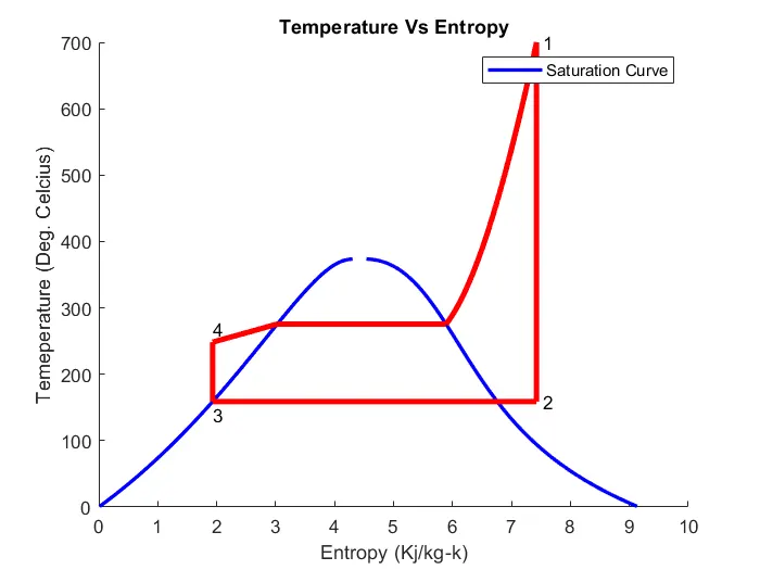
% Plotting T-S Diagram for Rankine Cycle
figure(1)
hold on
plot(sf,T,'color','b','linewidth',2)
plot(sg,T,'color','b','linewidth',2)
plot([s1 s2],[T1 T2], 'color', 'r', 'linewidth',3)
plot([s2 s3],[T2 T3], 'color', 'r', 'linewidth',3)
plot([s3 s4],[T3 T4], 'color', 'r', 'linewidth',3)
plot([s4 s5],[T4 T5], 'color', 'r', 'linewidth',3)
plot([s5 s6],[T5 T6], 'color', 'r', 'linewidth',3)
s_1 = linspace(s6,s1,1000);
for j = 1:length(s_1)
    Tc(j) = XSteam('T_ps',p1,s_1(j));
end
plot(s_1,Tc,'color','r','linewidth',3)
text(s1+0.1, T1, '1')
text(s2+0.1, T2, '2')
text(s3, T3-20, '3')
text(s4, T4+20, '4')
title('Temperature Vs Entropy')
xlabel('Entropy (Kj/kg-k)')
ylabel('Temeperature (Deg. Celcius)')
legend('Saturation Curve')

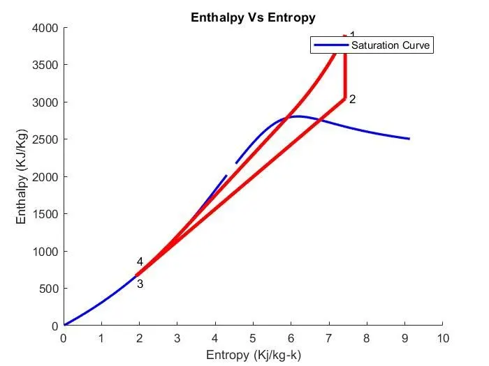
% Plotting H-S Diagram for Rankine Cycle
figure(2)
hold on
plot(sf,hf,'color','b','linewidth',2)
plot(sg,hg,'color','b','linewidth',2)
plot([s1 s2],[h1 h2],'color','r','linewidth',3)
plot([s2 s3],[h2 h3],'color','r','linewidth',3)
plot([s3 s4],[h3 h4],'color','r','linewidth',3)
hc = linspace(h4,h5,100);
for k = 1:length(hc)
    s_c(k) = XSteam('s_ph',p1,hc(k));
end
plot(s_c,hc,'color','r','linewidth',3)
plot([s5 s6],[h5 h6],'color','r','linewidth',3)
for l = 1:length(s_1)
    h_c(l) = XSteam('h_ps',p1,s_1(l));
end
plot(s_1,h_c,'color','r','linewidth',3)
text(s1+0.1,h1,'1')
text(s2+0.1,h2,'2')
text(s3,h3-100,'3')
text(s4,h4+200,'4')
title('Enthalpy Vs Entropy')
xlabel('Entropy (Kj/kg-k)')
ylabel('Enthalpy (KJ/Kg)')
legend('Saturation Curve')

% Displaying Results in Command window
disp('Results of Rankine Cycle')
fprintf('At state point 1\t\t\t\t\t')
fprintf('At state Point 2\n')
fprintf('P1 = %10f in Bar\t\t\t\t',p1);
fprintf('P2 = %10f in Bar\n',p2);
fprintf('T1 = %11f in Deg.Celcius\t\t',T1);
fprintf('T2 = %11f in Deg.Celcius\n',T2);
fprintf('H1 = %12f in KJ/Kg\t\t\t',h1);
fprintf('H2 = %12f in KJ/Kg\n',h2);
fprintf('S1 = %9f in KJ/Kg-k\t\t\t',s1);
fprintf('S2 = %9f in KJ/Kg-k\n',s2);
fprintf('\n')
fprintf('At state point 3\t\t\t\t\t')
fprintf('At state Point 4\n')
fprintf('P3 = %10f in Bar\t\t\t\t',p3);
fprintf('P4 = %10f in Bar\n',p4);
fprintf('T3 = %11f in Deg.Celcius\t\t',T3);
fprintf('T4 = %11f in Deg.Celcius\n',T4);
fprintf('H3 = %12f in KJ/Kg\t\t\t',h3);
fprintf('H4 = %12f in KJ/Kg\n',h4);
fprintf('S3 = %9f in KJ/Kg-k\t\t\t',s3);
fprintf('S4 = %9f in KJ/Kg-k\n',s4);
fprintf('\n')
fprintf('Turbine Work Done = %14f in KJ/Kg\n',W_T)
fprintf('Pump Work Done = %15f in KJ/Kg\n',W_P)
fprintf('Net Work Done  = %17f in KJ/Kg\n',W_net)
fprintf('Thermal Efficiency = %13f in percent\n',T_efficiency)
fprintf('Sp. Steam Consumption = %f in KJ/Kw\n',Sp_S)