Project 2 - Rankine cycle Simulator
The following code gives the Ideal Rankine Cycle Simulator
Aim: To create a ideal Rankine Cycle Simulator using OCTAVE/MATLAB.
PLATFORM USED :-
- Software – MATLAB R2019a
- Programming Language – C/C++
SYSTEM SPECIFICATIONS :-
- Manufacturer - DELL
- Model – Vostro 3478
- Operating System - Windows 10
- Processor - Intel(R) Core(TM) i5-8250U CPU @ 1.60GHz 1.80GHz
- RAM – 8 GB
OBJECTIVE :-
- To plot H-S and T-S diagram of Ideal Rankine Cycle.
- Evaluate the Net Work Done and Cycle Efficiency.
THEORY :-
The Rankine cycle is a model used to predict the performance of steam turbine systems. It was also used to study the performance of reciprocating steam engines. The Rankine cycle is an idealized thermodynamic cycle of a heat engine that converts heat into mechanical work while undergoing phase change. It is named after William John Macquorn Rankine, a Scottish polymath and Glasgow University professor.
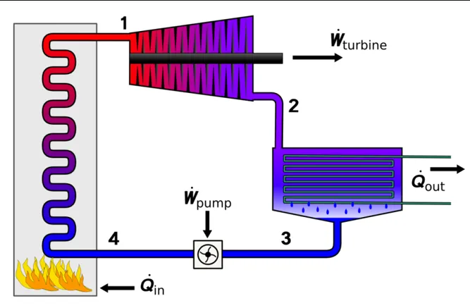
There are four process in Rankine Cycle,
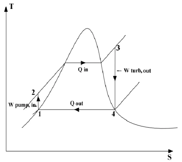
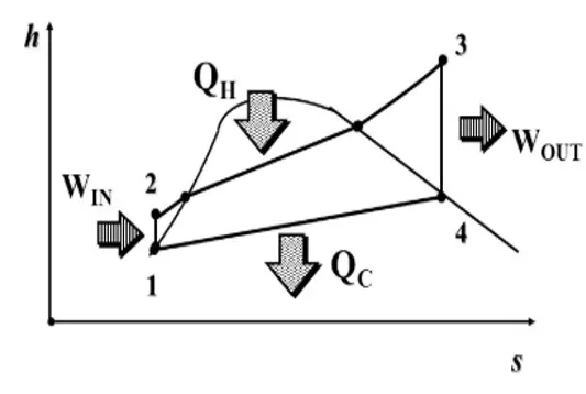
- Process 1-2 : Isentropic Compression in Pump
- Process 2-3 : Constant Pressure Heat Addition by the Boiler
- Process 3-4 : Isentropic Expansion in Turbine
- Process 4-1 : Constant Pressure Heat Rejection by the Condenser
PROCESS 1-2 :-
In this process the water is pumped to the boiler where the entropies remain constant (S1 = S2).
PROCESS 2-3 :-
In this process the boiler heats the pumped water and the state gets converted into steam at constant pressure (P2 = P3).
PROCESS 3-4 :-
In this process the steam gets expanded in the turbine to generate power where the entropies remain constant (S3 = S4).
PROCESS 4-1 :-
In this process the steam gets converted back into water by removing the heat from the steam at constant pressure (P4 = P1).
NOTE :-
Here I had considered that the Ideal Rankine Cycle starts from Turbine and ends in Boiler for easy calculations and plotting graphs. And also the formulae subject to change as the state points vary.
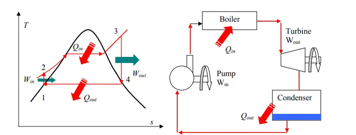
Energy Analysis
All four componenets of the Rankine cycle are steady-state staedy flow devices. The potentia and kinetic energy effects are neglected. The first law per unit mass of steam can be written as:
| Pump | q=0 |
W(pump.in)=h2-h1 |
| Boiler | w=0 | q(in)=h3-h2 |
| Turbine | q=0 | W(turbine.out)=h3-h4 |
| Condenser | w=0 | q(out)=h4-h1 |
Governing Equations
GOVERNING EQUATIONS :-
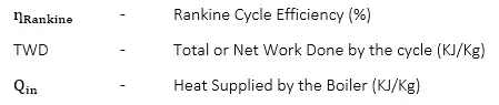
i.Efficiency of Rankine Cycle,
ƞRank=TWDHeat_SuppliedƞRank=TWDHeat_Supplied
Where,
ii.Work Done by the Turbine,
WTurb=H1–H2WTurb=H1–H2
Where,

iii.Work Done by the Pump,
WPump=H4–H3WPump=H4–H3
Where,

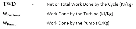
iv.Net Work Done,
TWD=WTurb−WPumpTWD=WTurb-WPump
Where,
v.Heat Supplied,
Qadd=H1–H4Qadd=H1–H4
Where,

vii.Heat Rejected,
Qout=H2–H3Qout=H2–H3
Where,

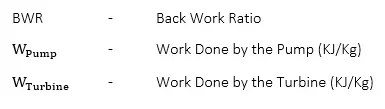
viii.Back Work Ratio,
BWR=WPumpWTurbBWR=WPumpWTurb
Where,
ix.Specific Steam Consumption,
SSC=3600WTurbSSC=3600WTurb
Where,

Main code
PROGRAM PROCESS :-
- The compiler starts the program.
- The Rankine Cycle process chart is printed
- The values of P1,T1 and P2 are obtained from the user.
- Next the H1 and S1 for state point 1 are calculated.
- Then H2,T2 and S2 for state point 2 are calculated.
- Next P3,T3,H3 and S3 for state point 3 are calculated.
- Next P4,T4,H4 and S4 for state point 4 are calculated
- Next T5,T6,S5 and S6 values are calculated.
- Turbine and Pump work done are evaluated.
- Net work done is evaluated.
- Heat added and rejected are evaluated.
- Thermal Efficiency, back work ratio and specific steam consumption are evaluated.
- Next the values of S, T, P and H are displayed for all the four state points.
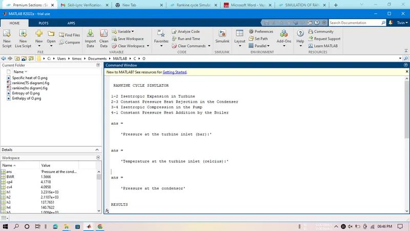
- Also, the Rankine Cycle parameters are displayed in the command window.
- Next the H-S and T-S diagram are plotted.
- The compiler terminates the program.
Step-wise explanation:
Function X-steam is used, which is the steam table
- Clearing the command window, workspace, and closing all plots
- Print description of all processes in the command window.
- Give the required inputs p1, T1, and p2.
- Defining the specific heat(Cp) for values for liquid and vapour using the Xsteam function (steam table).
- Defining the saturation temperature Tsat using Xsteam.
- Defining saturation properties specific Enthalpy an Entropy at states 1, 2, 3, 4 using the Xsteam function and required inputs.
- Starting with the calculation of properties at states 1, 2, 3, 4 using Xstaem and required inputs.
- Calculate enthalpies H1, H2, H3, H4 at states 1, 2, 3, 4 using Xsteam.
- Calculate entropies S1, S2, S3, S4 at states 1, 2, 3, 4.
- Calculate the values of T2, T3, and Wp(pump work), to calculate H and S at different states.
- Now define a range of temperature using the linspace command required to plot the graph.
- Now define the values of enthalpy and entropy of liquid and vapour lines.
- Now coming to plotting, start with the T-S diagram plot all the property lines
- Plot the H-S diagram.
- Then calculate net work done, thermal efficiency, and SSC.
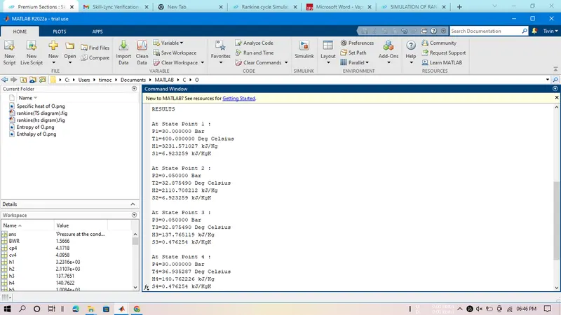
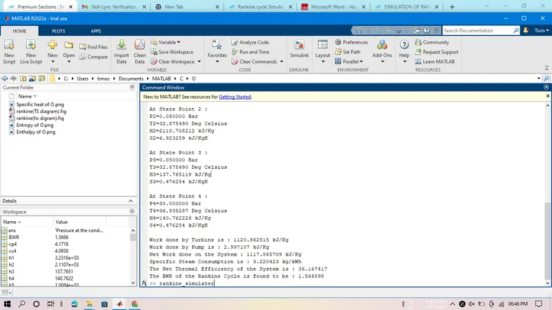
Results from Command Window
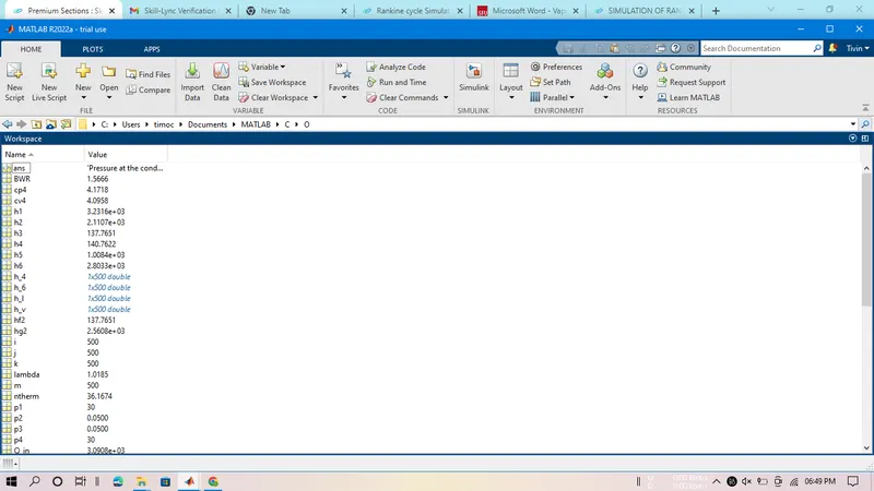
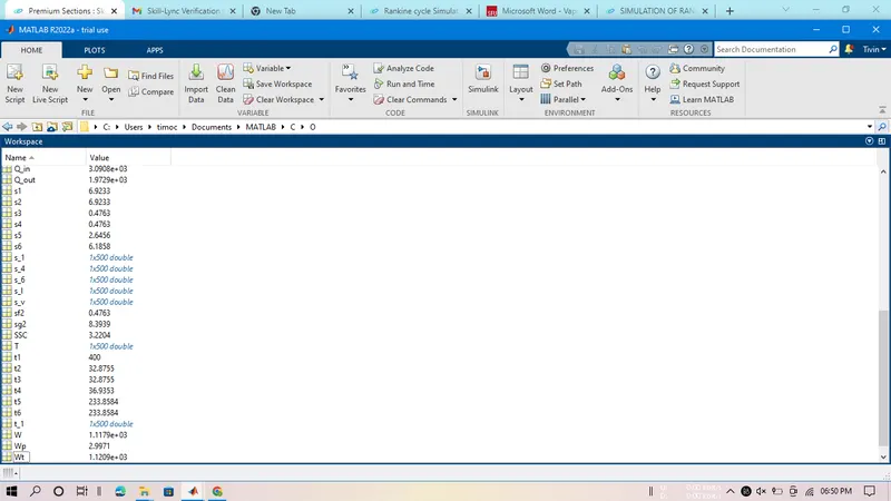
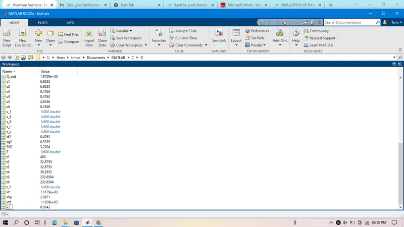
Results from Workspace
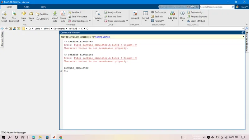
Errors faced
- The error will arise if we do not properly define the correct variables while giving the input.
This can be corrected by properly defining the input variable.
Plots are attached below (by running the rankine cycle simulator)
Results
Specific enthalpy and entropy values are calculated for different states and T-S and H-S diagrams are plotted